Multi-Channel EGG Analysis: A Complete Pipeline Tutorial#

This tutorial walks through the full analysis workflow for a multi-electrode electrogastrography (EGG) recording. It builds on the single-channel EGG Processing Tutorial and demonstrates the artefact-robust preprocessing methods introduced by Dalmaijer (2025).

By the end of this tutorial you will be able to:

Load and visualise a 7-channel EGG recording
Assess channel quality and select the optimal electrode
Apply spike removal, movement filtering, and bandpass cleaning
Compare the three multichannel strategies — per_channel, best_channel, and ica
Quantitatively compare outputs across methods with plots and tables
Fit a sine model to characterise the gastric oscillation

Prerequisites: EGG Processing Tutorial

Dataset: 7-electrode EGG from Wolpert et al. (2020), sampled at 10 Hz (∼12.6 min, fasted state).

Background#

Why use multiple electrodes?#

A single surface electrode picks up a spatially averaged view of the gastric slow wave (∼3 cpm / 0.05 Hz). Because the signal is small (∼50–500 µV at the skin surface) and easily contaminated by cardiac, respiratory, and motion artefacts, one electrode is often insufficient.

A multi-electrode array provides three complementary advantages:

Strategy	Benefit
Channel selection	Pick the electrode with the strongest gastric-band power (reduces noise floor)
Ensemble averaging	Summarise metrics across all electrodes to get a more stable estimate
Spatial denoising (ICA)	Decompose correlated artefacts into independent components and remove them

Electrode placement (Wolpert 2020)#

The bundled dataset uses a 7-electrode grid on the epigastric region. The stomach projects most strongly to midline electrodes, but signal quality varies by subject and recording condition.

Processing pipeline overview#

Raw multi-channel EGG
        │
        ▼
1. Visualise all channels — identify obvious problems
        │
        ▼
2. Channel quality assessment (Welch PSD → select best)
        │
        ▼
3. Artefact-robust preprocessing (Hampel + LMMSE + IIR)
        │
        ▼
4. Multichannel strategy: per_channel / best_channel / ica
        │
        ▼
5. Compare outputs → select for downstream analysis
        │
        ▼
6. Sine fitting for amplitude and phase characterisation

import warnings

import matplotlib.pyplot as plt
import numpy as np
from sklearn.exceptions import ConvergenceWarning

import gastropy as gp

plt.rcParams["figure.dpi"] = 100
plt.rcParams["figure.facecolor"] = "white"

print(f"GastroPy {gp.__version__}")

GastroPy 0.1.0

egg      = gp.load_egg()
signal   = egg["signal"]           # (7, n_samples)
sfreq    = egg["sfreq"]            # 10.0 Hz
ch_names = list(egg["ch_names"])
times    = np.arange(signal.shape[1]) / sfreq

print(f"Source   : {egg['source']}")
print(f"Channels : {signal.shape[0]}  ({ch_names})")
print(f"Samples  : {signal.shape[1]}  ({signal.shape[1]/sfreq:.0f} s,  "
      f"{signal.shape[1]/sfreq/60:.1f} min)")
print(f"Fs       : {sfreq} Hz")

Source   : wolpert_2020
Channels : 7  ([np.str_('EGG1'), np.str_('EGG2'), np.str_('EGG3'), np.str_('EGG4'), np.str_('EGG5'), np.str_('EGG6'), np.str_('EGG7')])
Samples  : 7580  (758 s,  12.6 min)
Fs       : 10.0 Hz

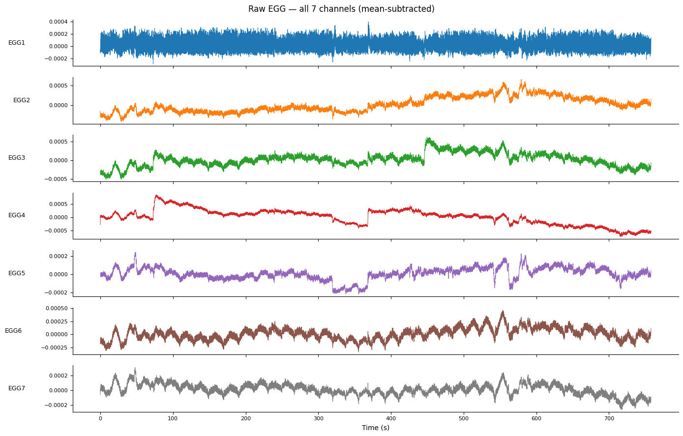
n_ch   = signal.shape[0]
colors = plt.cm.tab10(np.linspace(0, 0.7, n_ch))

fig, axes = plt.subplots(n_ch, 1, figsize=(14, 9), sharex=True)

for ax, ch, name, color in zip(axes, signal, ch_names, colors):
    ax.plot(times, ch - ch.mean(), lw=0.7, color=color)
    ax.set_ylabel(name, rotation=0, labelpad=40, va="center", fontsize=9)
    ax.tick_params(labelsize=8)
    for spine in ("top", "right"):
        ax.spines[spine].set_visible(False)

axes[-1].set_xlabel("Time (s)")
fig.suptitle("Raw EGG — all 7 channels (mean-subtracted)", fontsize=12)
fig.tight_layout()
plt.show()

../_images/466b45b35b1675f1024f07f8f8a731e7f4eab1a57bb8c9bebc7103b172c8e504.png

1. Channel Quality Assessment#

Before processing, it is important to identify which electrodes carry a reliable gastric signal. select_best_channel ranks channels by peak power in the normogastric band (2–4 cpm) using the Welch PSD method, following Wolpert et al. (2020).

When does channel quality matter?

For method="best_channel": the result depends entirely on this ranking.
For method="ica": high-quality channels provide better ICA mixing matrix estimates, reducing reconstruction artefacts.
For any single-channel downstream step: always start from the best channel.

# Compute Welch PSD for all channels
psd_list  = []
freqs_all = None
for ch in signal:
    freqs_ch, psd_ch = gp.psd_welch(ch, sfreq)
    psd_list.append(psd_ch)
    freqs_all = freqs_ch
psd_matrix = np.array(psd_list)   # (n_channels, n_freqs)

# Select the best channel
best_idx, peak_freq_hz, _, _ = gp.select_best_channel(signal, sfreq)
best_signal = signal[best_idx]

print(f"Best channel  : {ch_names[best_idx]}  (index {best_idx})")
print(f"Peak frequency: {peak_freq_hz:.4f} Hz  ({peak_freq_hz * 60:.2f} cpm)")
print()
print("Per-channel peaks:")
for i, name in enumerate(ch_names):
    _, pf, _, _ = gp.select_best_channel(signal[i : i + 1], sfreq)
    marker = "  ← best" if i == best_idx else ""
    print(f"  {name}: {pf:.4f} Hz  ({pf * 60:.2f} cpm){marker}")

Best channel  : EGG6  (index 5)
Peak frequency: 0.0530 Hz  (3.18 cpm)

Per-channel peaks:
  EGG1: 0.0520 Hz  (3.12 cpm)
  EGG2: 0.0380 Hz  (2.28 cpm)
  EGG3: 0.0520 Hz  (3.12 cpm)
  EGG4: 0.0350 Hz  (2.10 cpm)
  EGG5: 0.0370 Hz  (2.22 cpm)
  EGG6: 0.0530 Hz  (3.18 cpm)  ← best
  EGG7: 0.0530 Hz  (3.18 cpm)

fig, ax = plt.subplots(figsize=(10, 4))
gp.plot_psd(freqs_all, psd_matrix, ch_names=ch_names, best_idx=best_idx,
            peak_freq=peak_freq_hz, ax=ax)
plt.tight_layout()
plt.show()

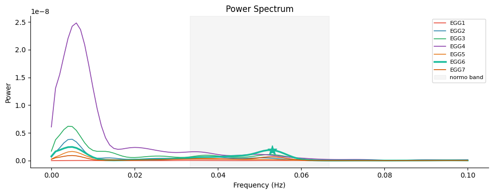
../_images/4a53c6b07265166a25781385957737c8cb140a92cfc88ec4cc6d5421de96349f.png

Interpreting the PSD#

The highlighted channel (EGG6) shows the clearest peak in the normogastric band (shaded region). Several observations are typical of multi-electrode EGG:

Signal variability across channels: channels closer to the stomach antrum typically show stronger gastric peaks; lateral or cephalad electrodes may show attenuated or shifted peaks.
Low-frequency drift (< 1 cpm): common in prolonged fasted recordings, usually due to respiration or electrode drift — removed by bandpass filtering.
Secondary peaks at 2× the fundamental (≈ 6 cpm): harmonic content from the non-sinusoidal waveform shape of the gastric slow wave.

2. Artefact-Robust Preprocessing#

Raw EGG signals often contain two types of non-physiological contamination before bandpass filtering:

Artefact type	Cause	Recommended filter
Spike / transient	Electrode movement, static discharge	`hampel_filter`
Movement noise	Breathing, posture shifts, ambulatory motion	`remove_movement_artifacts`

GastroPy provides three named cleaning pipelines via egg_clean:

"fir" (default) — zero-phase FIR bandpass only; assumes the signal is already artefact-free.
"iir" — zero-phase IIR Butterworth bandpass; faster, slightly less sharp roll-off.
"dalmaijer2025" — full Dalmaijer (2025) pipeline: Hampel → LMMSE movement filter → IIR Butterworth. Recommended for ambulatory recordings.

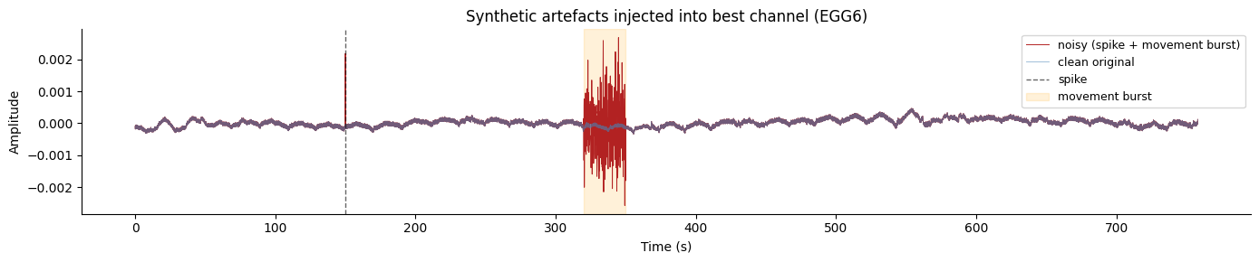
In this section we inject synthetic artefacts into the best channel and compare how "fir" and "dalmaijer2025" handle them.

rng = np.random.default_rng(42)

noisy = best_signal.copy()

# Inject a large spike (isolated sample, 20× signal amplitude)
spike_idx = 1500
noisy[spike_idx] += 20 * np.std(best_signal)

# Inject a sustained movement burst (300 samples, 8× signal SD)
burst_start, burst_end = 3200, 3500
noisy[burst_start:burst_end] += 8 * np.std(best_signal) * rng.standard_normal(
    burst_end - burst_start
)

fig, ax = plt.subplots(figsize=(14, 3))
ax.plot(times, noisy - noisy.mean(), lw=0.7, color="firebrick",
        label="noisy (spike + movement burst)")
ax.plot(times, best_signal - best_signal.mean(), lw=0.6, color="steelblue",
        alpha=0.6, label="clean original")
ax.axvline(times[spike_idx], color="black", lw=1, ls="--", alpha=0.6, label="spike")
ax.axvspan(times[burst_start], times[burst_end], alpha=0.15, color="orange",
           label="movement burst")
ax.set_xlabel("Time (s)")
ax.set_ylabel("Amplitude")
ax.set_title("Synthetic artefacts injected into best channel (EGG6)")
ax.legend(fontsize=9)
for spine in ("top", "right"):
    ax.spines[spine].set_visible(False)
plt.tight_layout()
plt.show()

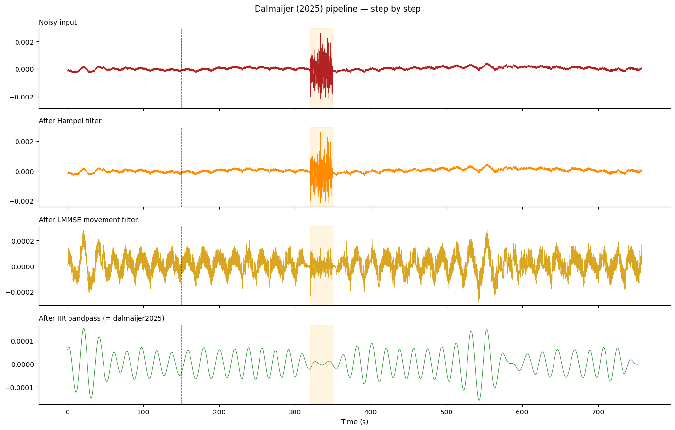
../_images/20e7e19735cf8956258fc3d05155a178a319583bfa67ab91fcca9522f474f868.png

# Step 1: Hampel spike removal (local sliding-window median replacement)
after_hampel = gp.hampel_filter(noisy)

# Step 2: LMMSE movement filter (Gharibans et al. 2018)
after_movement = gp.remove_movement_artifacts(after_hampel, sfreq)

# Step 3: IIR Butterworth bandpass
after_bandpass, _ = gp.egg_clean(after_movement, sfreq, method="iir")

stages = [
    ("Noisy input", noisy, "firebrick"),
    ("After Hampel filter", after_hampel, "darkorange"),
    ("After LMMSE movement filter", after_movement, "goldenrod"),
    ("After IIR bandpass (= dalmaijer2025)", after_bandpass, "forestgreen"),
]

fig, axes = plt.subplots(len(stages), 1, figsize=(14, 9), sharex=True)
for ax, (title, sig, color) in zip(axes, stages):
    ax.plot(times, sig - sig.mean(), lw=0.7, color=color)
    ax.set_title(title, fontsize=10, loc="left")
    ax.axvline(times[spike_idx], color="black", lw=0.8, ls="--", alpha=0.5)
    ax.axvspan(times[burst_start], times[burst_end],
               alpha=0.12, color="orange")
    for spine in ("top", "right"):
        ax.spines[spine].set_visible(False)

axes[-1].set_xlabel("Time (s)")
fig.suptitle("Dalmaijer (2025) pipeline — step by step", fontsize=12)
fig.tight_layout()
plt.show()

../_images/97b30d37047a0e91c018a65eb32178cf7ae7a1b3e7b98e0c9f013e8069e9b109.png

# Compare the two main cleaning approaches on the noisy signal
cleaned_fir, info_fir   = gp.egg_clean(noisy, sfreq, method="fir")
cleaned_d25, info_d25   = gp.egg_clean(noisy, sfreq, method="dalmaijer2025")
cleaned_orig, _         = gp.egg_clean(best_signal, sfreq, method="fir")  # reference

print("FIR info     :", {k: v for k, v in info_fir.items() if not isinstance(v, np.ndarray)})
print("D25 info     :", {k: v for k, v in info_d25.items() if not isinstance(v, np.ndarray)})

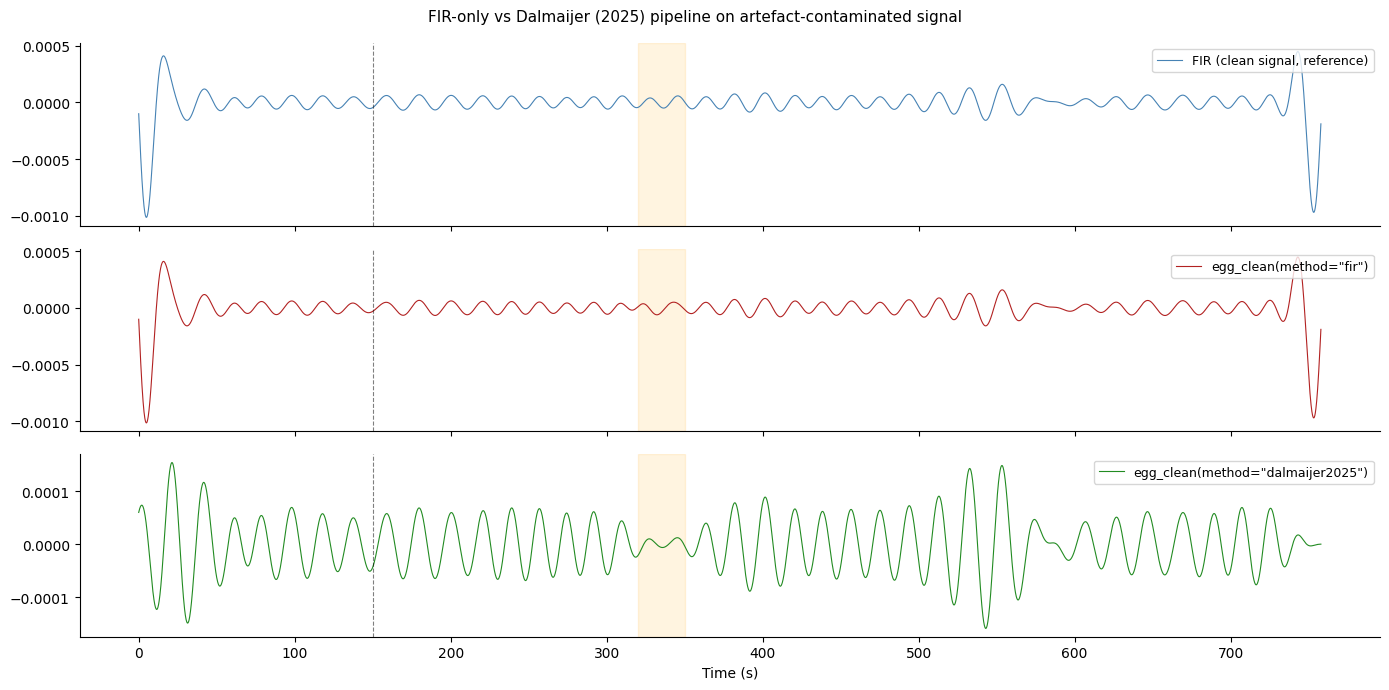
fig, axes = plt.subplots(3, 1, figsize=(14, 7), sharex=True)

axes[0].plot(times, cleaned_orig,  lw=0.8, color="steelblue",   label="FIR (clean signal, reference)")
axes[1].plot(times, cleaned_fir,   lw=0.8, color="firebrick",   label='egg_clean(method="fir")')
axes[2].plot(times, cleaned_d25,   lw=0.8, color="forestgreen", label='egg_clean(method="dalmaijer2025")')

for ax in axes:
    ax.axvline(times[spike_idx], color="black", lw=0.8, ls="--", alpha=0.5)
    ax.axvspan(times[burst_start], times[burst_end], alpha=0.12, color="orange")
    ax.legend(fontsize=9, loc="upper right")
    for spine in ("top", "right"):
        ax.spines[spine].set_visible(False)

axes[-1].set_xlabel("Time (s)")
fig.suptitle('FIR-only vs Dalmaijer (2025) pipeline on artefact-contaminated signal',
             fontsize=11)
fig.tight_layout()
plt.show()

FIR info     : {'filter_method': 'fir', 'fir_numtaps': 501, 'fir_window': 'hann', 'filtfilt_method': 'gust', 'cleaning_method': 'fir'}
D25 info     : {'cleaning_method': 'dalmaijer2025', 'hampel_k': 3, 'hampel_n_sigma': 3.0, 'movement_window': 1.0, 'freq_centre_hz': 0.049995, 'filter_method': 'iir_butter', 'butter_order': 4}

../_images/03d46c65ee56357c8579587975c39cf4264ce0601ca8f3896472ee5031ae9d24.png

Which cleaning pipeline should you use?#

Scenario	Recommended `method`
Clean lab recording, no visible spikes or movement	`"fir"` (default)
Occasional electrode pops or transient spikes	`"fir"` + manual inspection, or `"dalmaijer2025"`
Ambulatory recording (walking, exercise)	`"dalmaijer2025"`
Real-time or iterative processing	`"iir"`

Key observation from the plot above: method="fir" passes the spike and movement burst through to the output (they are broadband and land partly inside the filter passband). method="dalmaijer2025" attenuates both, recovering a trace close to the clean reference.

3. Multichannel Processing Strategies#

egg_process_multichannel applies one of three named strategies to a (n_channels, n_samples) array. The strategies differ in how they combine spatial information across electrodes:

`method`	Spatial handling	Best for
`"per_channel"`	Independent; returns all-channel summary + best idx	Comparing electrodes; quality screening
`"best_channel"`	Select strongest channel; full `egg_process` on it	Single-channel metrics with automatic selection
`"ica"`	FastICA spatial denoising then per-channel	Noisy/ambulatory data; maximise SNR

We will run all three on the clean real signal below, then compare their outputs quantitatively.

result_per = gp.egg_process_multichannel(signal, sfreq, method="per_channel")

summary = result_per["summary"].copy()
summary.insert(1, "channel_name", ch_names)
print("per_channel summary:")
print(summary.to_string(index=False, float_format="{:.4g}".format))
print(f"\nBest channel (by band power): {ch_names[result_per['best_idx']]}  "
      f"(index {result_per['best_idx']})")

per_channel summary:
 channel channel_name  peak_freq_hz  instability_coefficient  proportion_normogastric  band_power_mean
       0         EGG1         0.052                   0.2115                   0.9211        2.388e-11
       1         EGG2         0.038                   0.3477                   0.8889        3.807e-10
       2         EGG3         0.052                   0.3595                   0.9143        6.718e-10
       3         EGG4         0.035                   0.1422                        1        8.955e-10
       4         EGG5         0.037                    1.408                    0.913        2.085e-10
       5         EGG6         0.053                   0.1759                   0.9459        8.264e-10
       6         EGG7         0.053                   0.7241                   0.9355        3.041e-10

Best channel (by band power): EGG4  (index 3)

result_best = gp.egg_process_multichannel(signal, sfreq, method="best_channel")

bi   = result_best["info"]["best_channel_idx"]
info = result_best["info"]
print(f"best_channel result:")
print(f"  Selected channel   : {ch_names[bi]}  (index {bi})")
print(f"  Peak frequency     : {info['peak_freq_hz']:.4f} Hz  "
      f"({info['peak_freq_hz'] * 60:.2f} cpm)")
print(f"  Proportion normo   : {info['proportion_normogastric']:.0%}")
print(f"  Instability coeff  : {info['instability_coefficient']:.4f}")
print(f"  Cycles detected    : {info['cycle_stats']['n_cycles']}")
print(f"  Mean cycle duration: {info['cycle_stats']['mean_cycle_dur_s']:.1f} s")

best_channel result:
  Selected channel   : EGG6  (index 5)
  Peak frequency     : 0.0530 Hz  (3.18 cpm)
  Proportion normo   : 95%
  Instability coeff  : 0.1759
  Cycles detected    : 37
  Mean cycle duration: 20.3 s

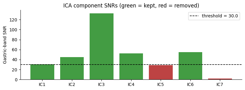
# ICA with a strict threshold (30.0) to demonstrate component removal.
# In practice, the default (3.0) is appropriate for most recordings.
with warnings.catch_warnings():
    warnings.simplefilter("ignore", ConvergenceWarning)
    result_ica = gp.egg_process_multichannel(
        signal, sfreq,
        method="ica",
        ica_snr_threshold=30.0,
        ica_random_state=42,
    )

ica_info = result_ica["ica_info"]
snrs     = ica_info["component_snr"]

print(f"ICA: {ica_info['n_components']} components total — "
      f"{ica_info['n_kept']} kept, {ica_info['n_removed']} removed "
      f"(threshold = {ica_info['snr_threshold']})")
print(f"Component SNRs: {snrs.round(2)}")
print()

ica_summary = result_ica["summary"].copy()
ica_summary.insert(1, "channel_name", ch_names)
print("ICA summary:")
print(ica_summary.to_string(index=False, float_format="{:.4g}".format))

ICA: 7 components total — 5 kept, 2 removed (threshold = 30.0)
Component SNRs: [ 30.39  44.94 132.53  52.32  28.79  54.93   2.33]

ICA summary:
 channel channel_name  peak_freq_hz  instability_coefficient  proportion_normogastric  band_power_mean
       0         EGG1         0.053                  0.09653                   0.9737        2.758e-12
       1         EGG2         0.038                   0.2487                   0.8947        5.154e-10
       2         EGG3         0.037                   0.3323                   0.9143        7.914e-10
       3         EGG4         0.035                   0.1441                        1        8.978e-10
       4         EGG5         0.037                    1.389                   0.7222         1.24e-10
       5         EGG6         0.053                   0.1766                   0.9459        8.303e-10
       6         EGG7         0.053                   0.7563                      0.9        2.727e-10

# Visualise ICA component SNRs with threshold line
fig, ax = plt.subplots(figsize=(8, 3))
x    = np.arange(len(snrs))
cols = ["forestgreen" if s >= ica_info["snr_threshold"] else "firebrick"
        for s in snrs]
ax.bar(x, snrs, color=cols, alpha=0.85)
ax.axhline(ica_info["snr_threshold"], color="black", lw=1.2, ls="--",
           label=f"threshold = {ica_info['snr_threshold']}")
ax.set_xticks(x)
ax.set_xticklabels([f"IC{i+1}" for i in x])
ax.set_ylabel("Gastric-band SNR")
ax.set_title("ICA component SNRs (green = kept, red = removed)")
ax.legend()
for spine in ("top", "right"):
    ax.spines[spine].set_visible(False)
plt.tight_layout()
plt.show()

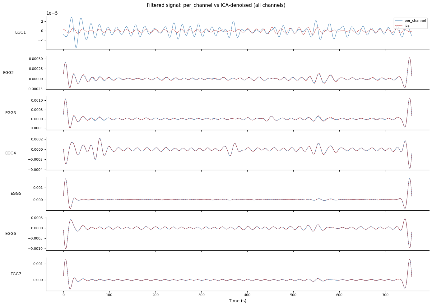
../_images/d00c25dfab7bc29299ea4287de578a7ba84e6866f64ef14e39654087c0eefb36.png

# Compare per_channel vs ICA-denoised filtered trace for every channel
fig, axes = plt.subplots(n_ch, 1, figsize=(14, 10), sharex=True)

for i, (ax, name, color) in enumerate(zip(axes, ch_names, colors)):
    per_filtered = result_per["channels"][i][0]["filtered"].values
    ica_filtered = result_ica["channels"][i][0]["filtered"].values

    ax.plot(times, per_filtered, lw=0.8, color="steelblue",   alpha=0.9,
            label="per_channel")
    ax.plot(times, ica_filtered, lw=0.9, color="firebrick", alpha=0.75,
            label="ica", ls="--")
    ax.set_ylabel(name, rotation=0, labelpad=40, va="center", fontsize=9)
    ax.tick_params(labelsize=8)
    for spine in ("top", "right"):
        ax.spines[spine].set_visible(False)

axes[0].legend(loc="upper right", fontsize=8)
axes[-1].set_xlabel("Time (s)")
fig.suptitle("Filtered signal: per_channel vs ICA-denoised (all channels)",
             fontsize=11)
fig.tight_layout()
plt.show()

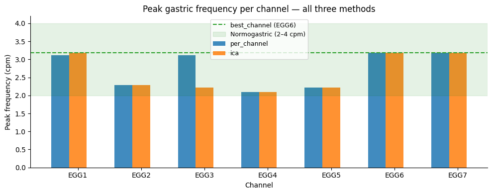
../_images/10bfae73f14e222a6bfd72fad9d78f64cfe7f516fc8ce67b1f2f9c2e71880c65.png

4. Comparing Methods#

Now we compare the three methods quantitatively.

Two questions:

Do the estimated peak frequencies agree across methods? High agreement suggests the gastric rhythm estimate is robust.
Does ICA change the stability and rhythmicity metrics? Meaningful changes indicate that component removal has attenuated non-gastric artefacts, sharpening the signal.

fig, ax = plt.subplots(figsize=(10, 4))

x = np.arange(n_ch)
w = 0.28

peak_per = result_per["summary"]["peak_freq_hz"].values * 60
peak_ica = result_ica["summary"]["peak_freq_hz"].values * 60

ax.bar(x - w, peak_per, width=w, label="per_channel", color="#1f77b4", alpha=0.85)
ax.bar(x,      peak_ica, width=w, label="ica",         color="#ff7f0e", alpha=0.85)
ax.axhline(result_best["info"]["peak_freq_hz"] * 60, color="#2ca02c",
           lw=1.5, ls="--",
           label=f"best_channel ({ch_names[result_best['info']['best_channel_idx']]})")

ax.axhspan(2, 4, alpha=0.1, color="green", label="Normogastric (2–4 cpm)")
ax.set_xticks(x)
ax.set_xticklabels(ch_names)
ax.set_xlabel("Channel")
ax.set_ylabel("Peak frequency (cpm)")
ax.set_title("Peak gastric frequency per channel — all three methods")
ax.legend(fontsize=9)
for spine in ("top", "right"):
    ax.spines[spine].set_visible(False)
plt.tight_layout()
plt.show()

../_images/e0c3ee8637441b48c26b9e35c27a1f7ff9cfee432f87658ffa97549dce474efd.png

import pandas as pd

# Build a side-by-side comparison table for all channels
rows = []
for i, name in enumerate(ch_names):
    per_info = result_per["channels"][i][1]
    ica_info_ch = result_ica["channels"][i][1]
    rows.append({
        "channel":        name,
        "IC (per_ch)":    per_info["instability_coefficient"],
        "IC (ica)":       ica_info_ch["instability_coefficient"],
        "normo% (per_ch)": per_info["proportion_normogastric"],
        "normo% (ica)":   ica_info_ch["proportion_normogastric"],
        "peak Hz (per_ch)": per_info["peak_freq_hz"],
        "peak Hz (ica)":  ica_info_ch["peak_freq_hz"],
    })

comparison = pd.DataFrame(rows)
print("Method comparison — instability coefficient, proportion normogastric, peak frequency:")
print(comparison.to_string(index=False, float_format="{:.4g}".format))

Method comparison — instability coefficient, proportion normogastric, peak frequency:
channel  IC (per_ch)  IC (ica)  normo% (per_ch)  normo% (ica)  peak Hz (per_ch)  peak Hz (ica)
   EGG1       0.2115   0.09653           0.9211        0.9737             0.052          0.053
   EGG2       0.3477    0.2487           0.8889        0.8947             0.038          0.038
   EGG3       0.3595    0.3323           0.9143        0.9143             0.052          0.037
   EGG4       0.1422    0.1441                1             1             0.035          0.035
   EGG5        1.408     1.389            0.913        0.7222             0.037          0.037
   EGG6       0.1759    0.1766           0.9459        0.9459             0.053          0.053
   EGG7       0.7241    0.7563           0.9355           0.9             0.053          0.053

When to use each strategy#

Strategy	Use when
`"per_channel"`	You want a quality overview of all electrodes; useful for QC, identifying bad channels, or summarising a group study
`"best_channel"`	You need a single-channel result with minimal configuration; equivalent to `select_best_channel` + `egg_process`
`"ica"`	Your recording has coherent spatial noise (ambulatory subjects, high-motion environments); short or very clean lab recordings see minimal benefit

Note on this dataset: The Wolpert et al. (2020) recording is a clean laboratory acquisition — participants were seated and fasted. ICA with the default snr_threshold=3.0 removes only 1 of 7 components (SNR=2.33), producing negligible changes to the metrics. For ambulatory recordings, the effect is typically much larger. We used snr_threshold=30.0 in cells above solely to illustrate what component removal looks like.

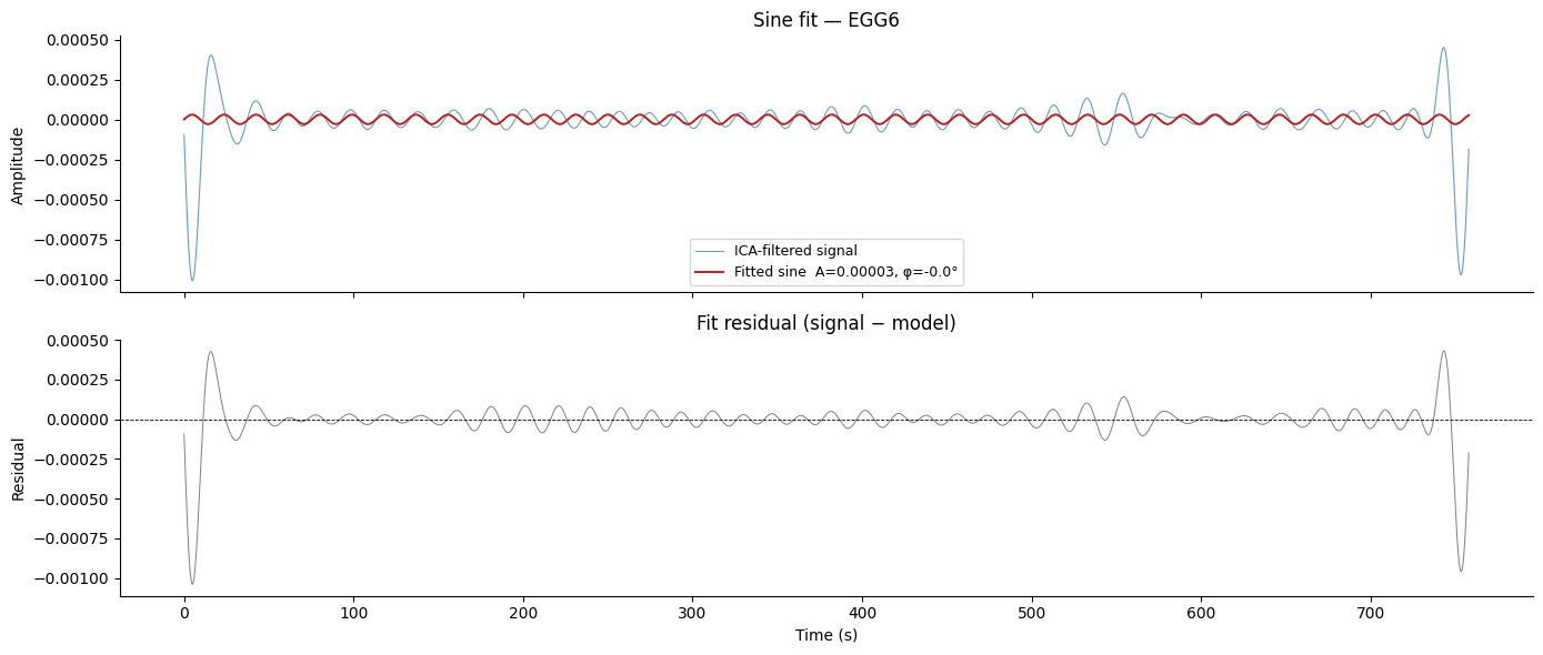
5. Sine Fitting#

Once we have a clean, bandpass-filtered gastric signal, fit_sine fits a sinusoidal model A · sin(2πft + φ) using L-BFGS-B least-squares optimisation (Dalmaijer, 2025).

Why fit a sine?

Provides a single amplitude estimate that is more robust than the envelope from the Hilbert transform for short recordings.
Gives a precise phase offset φ, directly interpretable for gastric–brain coupling experiments (e.g., aligning EEG epochs to the gastric phase at stimulus onset).
The residual quantifies how well the gastric rhythm approximates a pure sinusoid — useful as an additional quality metric.

# Use the ICA-denoised, filtered best channel
best_ica_filtered = result_ica["channels"][best_idx][0]["filtered"].values

# Fit with the known peak frequency locked in (faster, more stable)
sine_result = gp.fit_sine(best_ica_filtered, sfreq=sfreq, freq=peak_freq_hz)

print(f"Fitted to channel   : {ch_names[best_idx]}")
print(f"Fixed frequency     : {sine_result['freq_hz']:.4f} Hz  "
      f"({sine_result['freq_hz'] * 60:.2f} cpm)")
print(f"Fitted amplitude    : {sine_result['amplitude']:.6f}")
print(f"Fitted phase offset : {sine_result['phase_rad']:.4f} rad  "
      f"({np.degrees(sine_result['phase_rad']):.1f}°)")
print(f"Residual (SS)       : {sine_result['residual']:.4e}")

Fitted to channel   : EGG6
Fixed frequency     : 0.0530 Hz  (3.18 cpm)
Fitted amplitude    : 0.000030
Fitted phase offset : -0.0000 rad  (-0.0°)
Residual (SS)       : 1.4294e-04

t_vec     = np.arange(len(best_ica_filtered)) / sfreq
fitted    = gp.sine_model(t_vec,
                          freq=sine_result["freq_hz"],
                          phase=sine_result["phase_rad"],
                          amp=sine_result["amplitude"])
residual  = best_ica_filtered - fitted

fig, axes = plt.subplots(2, 1, figsize=(14, 6), sharex=True)

axes[0].plot(t_vec, best_ica_filtered, lw=0.8, color="steelblue",
             alpha=0.8, label="ICA-filtered signal")
axes[0].plot(t_vec, fitted, lw=1.4, color="firebrick",
             label=f"Fitted sine  A={sine_result['amplitude']:.5f}, "
                   f"φ={np.degrees(sine_result['phase_rad']):.1f}°")
axes[0].set_ylabel("Amplitude")
axes[0].set_title(f"Sine fit — {ch_names[best_idx]}")
axes[0].legend(fontsize=9)

axes[1].plot(t_vec, residual, lw=0.7, color="dimgrey", alpha=0.85)
axes[1].axhline(0, color="black", lw=0.6, ls="--")
axes[1].set_ylabel("Residual")
axes[1].set_xlabel("Time (s)")
axes[1].set_title("Fit residual (signal − model)")

for ax in axes:
    for spine in ("top", "right"):
        ax.spines[spine].set_visible(False)

plt.tight_layout()
plt.show()

../_images/6bd719b151b9e61235f375d1014c2a07af5135118dbede7bff334615bb0348a5.png

Summary#

This tutorial covered the complete multi-channel EGG analysis pipeline:

Workflow recap#

Step	Function	Key output
Load data	`gp.load_egg()`	`signal` (n_ch, n_samp)
Channel quality	`gp.select_best_channel()`	`best_idx`, `peak_freq_hz`
PSD visualisation	`gp.psd_welch()` + `gp.plot_psd()`	PSD plot
Spike removal	`gp.hampel_filter()`	Spike-free signal
Movement filtering	`gp.remove_movement_artifacts()`	Motion-corrected signal
Robust cleaning	`gp.egg_clean(method="dalmaijer2025")`	Fully preprocessed signal
All-channel processing	`gp.egg_process_multichannel(method="per_channel")`	Summary DataFrame
Optimal-channel processing	`gp.egg_process_multichannel(method="best_channel")`	`egg_process` result
Spatial denoising	`gp.egg_process_multichannel(method="ica")`	ICA-denoised metrics
Sine characterisation	`gp.fit_sine()`	Amplitude, phase, residual

References#

Dalmaijer, E. S. (2025). electrography v1.1.1. https://github.com/esdalmaijer/electrography
Gharibans, A. A., et al. (2018). Artifact rejection methodology enables continuous, noninvasive measurement of gastric myoelectric activity in ambulatory subjects. Scientific Reports, 8, 5019. https://doi.org/10.1038/s41598-018-23302-9
Wolpert, N., Rebollo, I., & Tallon-Baudry, C. (2020). Electrogastrography for psychophysiological research: Practical considerations, analysis pipeline, and normative data in a large sample. Psychophysiology, 57, e13599. https://doi.org/10.1111/psyp.13599

Multi-Channel EGG Analysis: A Complete Pipeline Tutorial

Contents