Time-Frequency Representation#

Compute and visualize a Morlet wavelet time-frequency representation of an EGG signal using morlet_tfr and plot_tfr. This is useful for examining how spectral power evolves over the recording.

The TFR performs its own frequency decomposition, so it should be applied directly to the raw EGG signal (no bandpass filtering needed).

import matplotlib.pyplot as plt
import numpy as np

import gastropy as gp

plt.rcParams["figure.dpi"] = 100
plt.rcParams["figure.facecolor"] = "white"

Load EGG Data#

Load the sample recording and select the best channel.

# Load sample EGG data
egg = gp.load_egg()
signal = egg['signal']
sfreq = egg['sfreq']
ch_names = list(egg['ch_names'])

# Select best channel
best_idx, peak_freq, _, _ = gp.select_best_channel(signal, sfreq)
raw = signal[best_idx]
times = np.arange(len(raw)) / sfreq

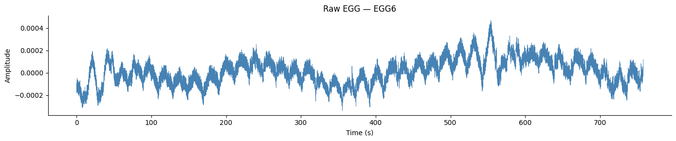
print(f"Best channel: {ch_names[best_idx]}, peak: {peak_freq * 60:.1f} cpm")
print(f"Recording duration: {times[-1]:.0f} s")

Best channel: EGG6, peak: 3.2 cpm
Recording duration: 758 s

Raw Signal#

fig, ax = plt.subplots(figsize=(14, 3))
ax.plot(times, raw - np.mean(raw), color='steelblue', linewidth=0.6)
ax.set_xlabel('Time (s)')
ax.set_ylabel('Amplitude')
ax.set_title(f'Raw EGG — {ch_names[best_idx]}')
ax.spines['top'].set_visible(False)
ax.spines['right'].set_visible(False)
fig.tight_layout()
plt.show()

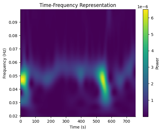
../_images/521e348c338b3ffa400c295f2589ae1fb264c3bcda89f468d8b11f31aee150b9.png

Basic TFR#

Compute the Morlet wavelet TFR across the gastric frequency range (0.02–0.1 Hz, i.e. 1–6 cpm). The function mean-centers and reflect-pads the signal internally to avoid edge artifacts.

freqs = np.arange(0.02, 0.1, 0.001)
freqs_out, tfr_times, power = gp.morlet_tfr(raw, sfreq=sfreq, freqs=freqs)

fig, ax = gp.plot_tfr(freqs_out, tfr_times, power)
plt.show()

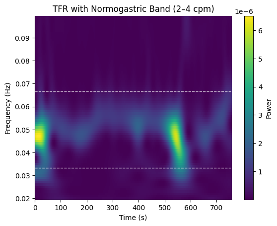
../_images/ccf9c8051bdc87a95987c131d84f547822ee1cdeeb1b5501a91d5c41d00eb32a.png

With Normogastric Band Overlay#

Pass a GastricBand to draw the band boundaries on the plot.

fig, ax = gp.plot_tfr(freqs_out, tfr_times, power, band=gp.NORMOGASTRIA)
ax.set_title("TFR with Normogastric Band (2\u20134 cpm)")
plt.show()

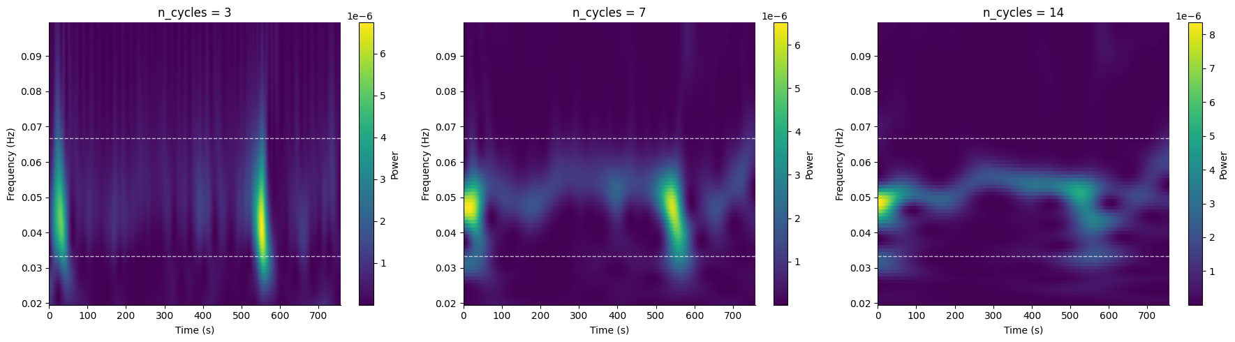
../_images/5b9c6e5381cdeb1a7ef2492bb634a54237982b8cf05b6981cc0e7bf2f5444725.png

Adjusting Time-Frequency Resolution#

The n_cycles parameter controls the trade-off between time and frequency resolution. Fewer cycles give better time resolution; more cycles give better frequency resolution.

fig, axes = plt.subplots(1, 3, figsize=(18, 5))

for ax, nc in zip(axes, [3, 7, 14], strict=True):
    _, _, pwr = gp.morlet_tfr(raw, sfreq=sfreq, freqs=freqs, n_cycles=nc)
    gp.plot_tfr(freqs, tfr_times, pwr, band=gp.NORMOGASTRIA, ax=ax)
    ax.set_title(f'n_cycles = {nc}')

fig.tight_layout()
plt.show()

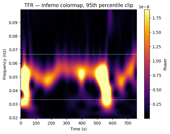
../_images/0889486020fe07169291868df531bc6b358b51c01b5de626a93e9891c06a2df0.png

Custom Colormap and Color Limits#

Use cmap, vmin, and vmax to customize the appearance.

fig, ax = gp.plot_tfr(
    freqs_out, tfr_times, power,
    band=gp.NORMOGASTRIA,
    cmap="inferno",
    vmax=np.percentile(power, 95),
)
ax.set_title("TFR — Inferno colormap, 95th percentile clip")
plt.show()

../_images/cc8458b03213ab2fe2adf24a8e41fbfaab8016d2e5989b4a106c4878e5f9702e.png

Time-Frequency Representation

Contents