Cycle Duration Histogram

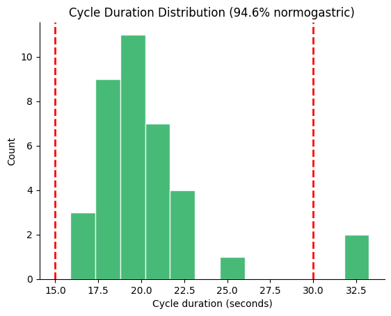
Visualize the distribution of gastric cycle durations using plot_cycle_histogram. The normogastric range (default 15–30 s) is marked with dashed lines, and the percentage of normogastric cycles is shown in the title.

import matplotlib.pyplot as plt

import gastropy as gp

plt.rcParams["figure.dpi"] = 100
plt.rcParams["figure.facecolor"] = "white"

# Load and process
egg = gp.load_egg()
best_idx, _, _, _ = gp.select_best_channel(egg["signal"], egg["sfreq"])
_, info = gp.egg_process(egg["signal"][best_idx], egg["sfreq"])
durations = info["cycle_durations_s"]
print(f"{len(durations)} cycles detected")

37 cycles detected

Default Normogastric Range (15–30 s)

fig, ax = gp.plot_cycle_histogram(durations)
plt.show()

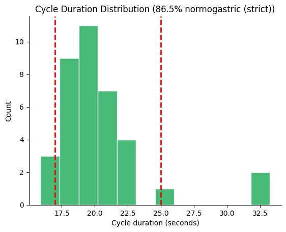
Custom Normogastric Range

Some studies use a narrower range (e.g., 17–25 s for ~2.4–3.5 cpm). Pass normo_range to adjust the boundary lines and percentage.

fig, ax = gp.plot_cycle_histogram(durations, normo_range=(17.0, 25.0))
ax.set_title(ax.get_title().replace("normogastric", "normogastric (strict)"))
plt.show()

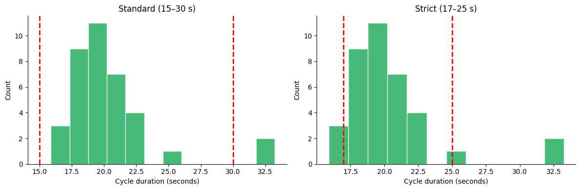
Side-by-Side Comparison

Pass an ax to embed the histogram in a custom figure layout.

fig, (ax1, ax2) = plt.subplots(1, 2, figsize=(12, 4))
gp.plot_cycle_histogram(durations, normo_range=(15.0, 30.0), ax=ax1)
ax1.set_title("Standard (15–30 s)")
gp.plot_cycle_histogram(durations, normo_range=(17.0, 25.0), ax=ax2)
ax2.set_title("Strict (17–25 s)")
fig.tight_layout()
plt.show()

See also: Quality Assessment, EGG Processing Tutorial