Metacognition

Author: Micah G. Allen

The Heart Rate Discrimination task records a confidence rating after every choice. These ratings let us ask whether participants know when their judgements are likely to be correct. This is a separate question from whether they can discriminate changes in heart rate.

The previous tutorial used faster and slower choices to estimate psychophysical bias, precision, and lapse rate. Here we fit a second hierarchical model in which confidence is the outcome. The principles of partial pooling and random effects remain the same, but the likelihood and the scientific interpretation are different.

Confidence bias and metacognitive calibration

We use the confidence ratings to distinguish two quantities.

• Confidence bias describes how participants use the rating scale. A participant may tend to report high or low confidence regardless of whether a response was correct.

• Metacognitive calibration describes the association between confidence and accuracy. In this tutorial, it is the difference in expected confidence between correct and incorrect trials.

These quantities can vary independently. A participant can be confident but poorly calibrated, or cautious while still assigning higher confidence to their correct responses. In the regression model, the intercept and other main effects describe confidence bias, while the coefficient for Accuracy describes calibration in the reference condition. Interactions with Accuracy test whether calibration changes across conditions or participant characteristics.

We reserve the terms metacognitive sensitivity and metacognitive efficiency for signal detection measures such as meta-d-prime and M-ratio. Ordered beta regression does not fit a signal detection model, so calibration is the more accurate name for the quantity estimated here.

The confidence distribution determines the likelihood

Confidence is recorded on a continuous slider from 0 to 100. Participants can select either endpoint, and those observations are meaningful. In the example data, 15.0% of ratings fall exactly on a bound, with 3.9% at zero and 11.1% at 100.

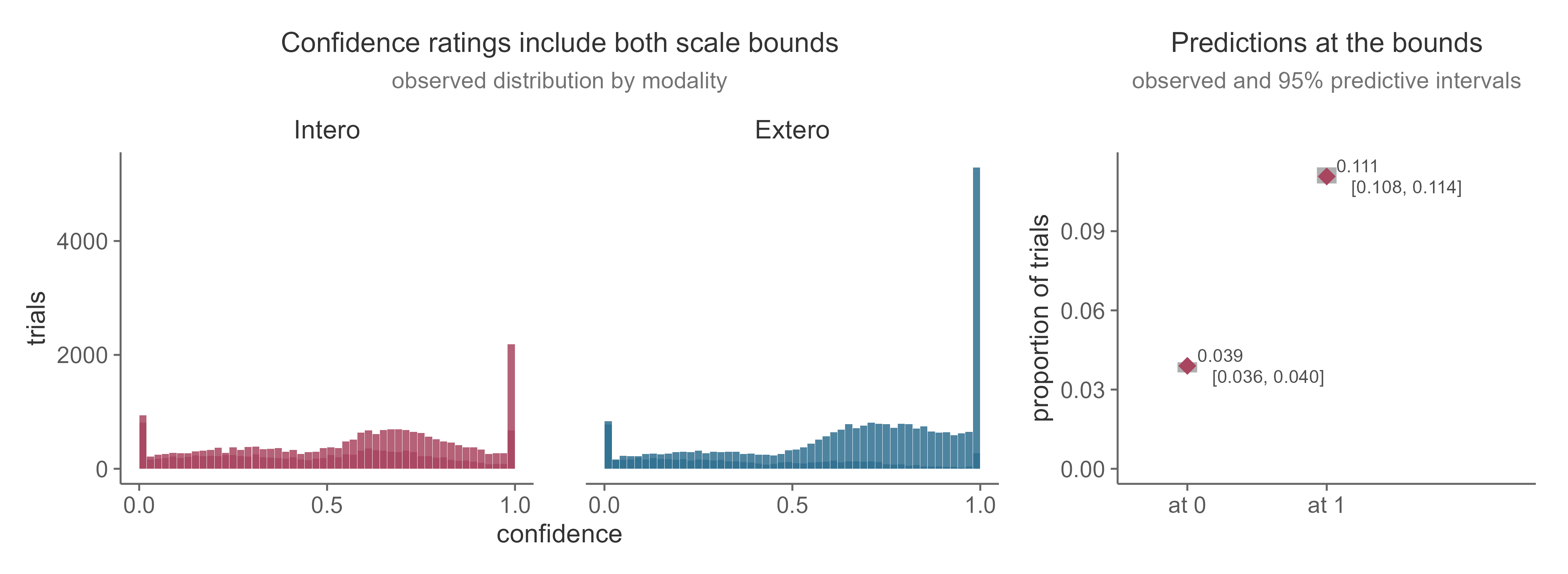
Several familiar likelihoods are poorly suited to these data.

Likelihood	Problem for HRD confidence
Gaussian	Assigns probability to values below 0 and above 1
Beta	Excludes observations at exactly 0 and 1
Ordinal after binning	Discards the resolution of the confidence slider

Ordered beta regression retains the continuous ratings and their exact bounds (Kubinec, 2023). It models zero, the open interval between zero and one, and one within a single likelihood. Two ordered cutpoints govern the probability of a response at either bound, while a beta distribution describes ratings in the interior. We therefore do not need to move endpoint ratings inward or convert the scale into categories.

The right panel above is an important posterior predictive check. A suitable model should reproduce both the interior distribution and the observed proportions at zero and one.

Why we do not use M-ratio for HRD data

M-ratio, defined as meta-d-prime divided by d-prime, is a useful measure of metacognitive efficiency for experiments that support its signal detection assumptions. The HRD design creates a specific problem for that analysis.

The Psi staircase places trials near each participant’s point of subjective equality. It is designed to estimate the cardiac bias described in the psychophysics tutorial, rather than to maintain a fixed level of objective accuracy. Accuracy is nevertheless scored relative to the participant’s measured heart rate. A faster response is correct above zero delta BPM, and a slower response is correct below zero.

Consider a participant with a threshold of -15 delta BPM. The staircase will present many trials near -15 because this is where their faster and slower responses are balanced. Most of those trials have slower as the objectively correct answer. The two stimulus classes required to estimate type 1 hit and false alarm rates are consequently very uneven. For participants with large cardiac biases, one class may contain only a few trials.

Under this design, d-prime also combines response bias with psychophysical precision. Dividing meta-d-prime by d-prime would reintroduce a distinction that the psychometric model was used to resolve. Finally, estimating meta-d-prime requires us to bin the continuous confidence ratings, making the result depend on arbitrary cutpoints.

This argument is specific to the task design. M-ratio remains appropriate for experiments with adequately sampled stimulus classes, suitable control over type 1 performance, and confidence ratings designed for an SDT analysis. For HRD, we model the trial-level confidence ratings directly and describe the accuracy-confidence association as metacognitive calibration.

Prepare trial-level confidence data

Begin with the trial data described in the inspection tutorial. Remove trials without a decision or confidence rating, preserve the exact slider endpoints, and code incorrect trials as the reference level.

library(dplyr)

confidence_data <- raw |>
  filter(
    Decision %in% c("More", "Less"),
    !is.na(Confidence),
    !is.na(ResponseCorrect)
  ) |>
  mutate(
    subj = factor(Subject),
    Accuracy = factor(
      if_else(
        tolower(as.character(ResponseCorrect)) %in% c("true", "1"),
        "correct",
        "incorrect"
      ),
      levels = c("incorrect", "correct")
    ),
    Modality = factor(Modality, levels = c("Extero", "Intero")),
    Confidence = Confidence / 100
  )

stopifnot(all(confidence_data$Confidence >= 0 &
              confidence_data$Confidence <= 1))

Do not recode a missed decision as incorrect. There is no choice to score on such a trial. Before fitting the model, inspect the range and scale use for each participant.

confidence_data |>
  group_by(subj) |>
  summarise(
    trials = n(),
    mean_confidence = mean(Confidence),
    sd_confidence = sd(Confidence),
    at_zero = mean(Confidence == 0),
    at_one = mean(Confidence == 1),
    .groups = "drop"
  )

A participant who selected one confidence value throughout the task provides no within-person information about calibration. Review these sessions before analysis and document any exclusion rule. Scale use is also worth plotting, because a standard deviation alone does not show whether a participant relied almost entirely on one endpoint.

The worked model also uses gender, age, and BMI. Set the gender reference level and join the participant-level standardized age and BMI variables prepared in the hierarchical modelling tutorial. Standardize these variables over one row per participant, rather than over the trial table.

Specify the hierarchical ordered beta model

A useful starting model is

Confidence ~ Accuracy + (Accuracy | subj)

The population coefficient for Accuracy estimates average metacognitive calibration. The participant intercepts allow confidence bias to vary, and the participant slopes allow the accuracy-confidence association to vary. Partial pooling regularizes both estimates.

The worked example extends this model to ask whether calibration differs between the cardiac and exteroceptive conditions, between genders, or with age. BMI is included as a covariate.

library(brms)
library(ordbetareg)

confidence_formula <- bf(
  Confidence ~ Accuracy * (Modality + gender + age_z) + bmi_z +
    (Accuracy * Modality | subj)
)

fit_confidence <- ordbetareg(
  formula = confidence_formula,
  data = confidence_data,
  chains = 4,
  cores = 4,
  control = list(adapt_delta = 0.95, max_treedepth = 12),
  file = "fit_confidence"
)

Accuracy and Modality vary within participants, so the model includes their random slopes and interaction. Gender, age, and BMI vary between participants and cannot receive participant-level random slopes. The same design rule is explained in the hierarchical modelling tutorial.

The worked model uses the package defaults for its priors. For a new study, use get_prior() to inspect the parameters created by your exact formula and carry out prior predictive checks before sampling. Ordered beta models can take several hours to fit, so cache the model with file and begin with a small test run to identify coding problems.

Interpret interactions through predictions

Regression coefficients are reported on the model’s latent scale. Their meaning also depends on the reference levels and interactions in the formula.

Term	Interpretation in the worked model
Accuracycorrect	Calibration for Extero trials among participants at the reference levels of the other predictors
ModalityIntero	Intero versus Extero difference on incorrect trials
Accuracycorrect:ModalityIntero	Change in calibration from Extero to Intero trials
age_z	Association between age and confidence on incorrect trials
Accuracycorrect:age_z	Association between age and calibration

The main effect of Modality is therefore not an overall modality difference, and the main effect of age is not an overall age effect. Once interactions are present, we should use posterior predictions to express the result on the confidence scale.

library(marginaleffects)

# Expected confidence for each accuracy by modality combination
avg_predictions(
  fit_confidence,
  by = c("Accuracy", "Modality")
)

# Correct minus incorrect confidence within each modality
avg_comparisons(
  fit_confidence,
  variables = "Accuracy",
  by = "Modality"
)

These summaries average over the requested observations. For a continuous moderator such as age, create a grid over the observed age range and plot the predictions for correct and incorrect trials. The distance between those lines is calibration.

Results from the worked model

The example model was fitted to 68,932 trials from 512 participants. The table shows selected population coefficients on the latent scale.

Term	Estimate	95% interval
Accuracycorrect	1.09	[1.03, 1.15]
ModalityIntero	0.36	[0.30, 0.41]
Accuracycorrect:ModalityIntero	-0.76	[-0.83, -0.70]
age_z	0.13	[0.08, 0.18]
Accuracycorrect:age_z	-0.02	[-0.06, 0.02]
genderMale	0.08	[-0.02, 0.19]
Accuracycorrect:genderMale	0.05	[-0.04, 0.13]

The response-scale predictions make these coefficients easier to interpret.

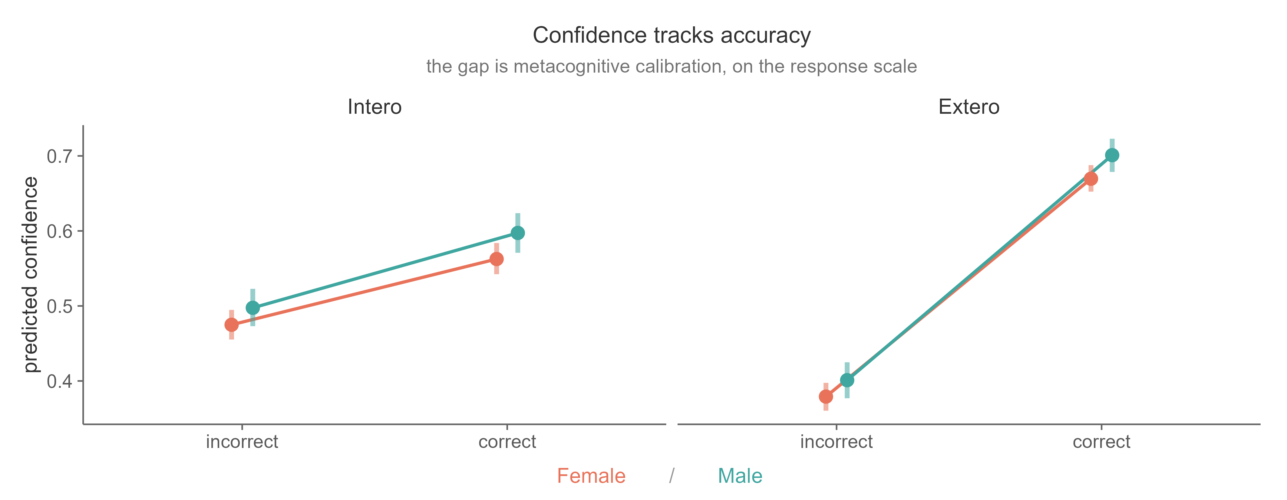
For women at the mean age and BMI, expected confidence on Extero trials was 0.67 after correct responses and 0.38 after incorrect responses. The calibration gap was therefore 0.29. On Intero trials, the corresponding predictions were 0.56 and 0.47, giving a gap of 0.09. The negative Accuracycorrect:ModalityIntero interaction captures this reduction in cardiac metacognitive calibration.

Notice how the modality comparison changes with accuracy. Predicted confidence was higher for Intero than Extero trials following an incorrect response, but lower following a correct response. Reporting ModalityIntero as an overall increase in cardiac confidence would miss this interaction. The estimated gender interaction was small and its interval included zero, so this analysis provides little evidence that calibration differed by gender.

Age and confidence bias

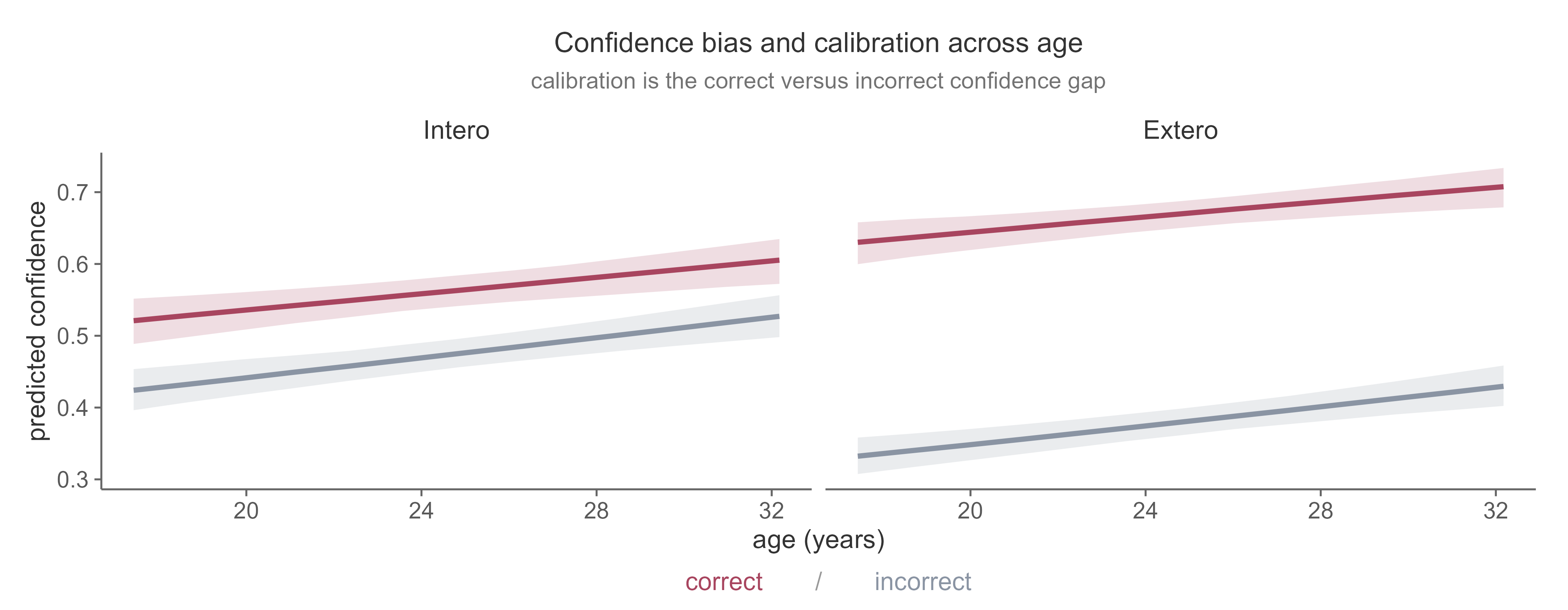
Expected confidence increased with age for both correct and incorrect trials. The two lines remained approximately parallel, and the interval for Accuracycorrect:age_z included zero. In this sample, age was associated with confidence bias but provided little evidence of a change in metacognitive calibration. This is why we examine the predicted confidence levels and their gap separately.

Check the fitted model

Begin with the standard sampling diagnostics. Check for divergent transitions, verify that R-hat is below 1.01, and inspect effective sample sizes and trace plots. If the model has convergence problems, do not interpret its coefficients.

Posterior predictive checks should then address the features that motivated the likelihood.

• Compare predicted and observed confidence distributions within each modality and accuracy condition.

• Compare the predicted and observed proportions at exactly zero and one.

• Check whether the model reproduces large differences in scale use between participants.

• Plot participant-level predictions to identify sessions that the population model describes poorly.

The first figure on this page illustrates the bound check. The observed proportions should fall within plausible posterior predictive intervals. A density plot of the interior ratings cannot establish this on its own.

Report the model and result

A clear report should state the number of participants and trials, the amount of confidence mass at both bounds, the fixed and random effect formula, the priors, and the sampling and posterior predictive diagnostics. Report the scientific result as response-scale expected confidence and calibration contrasts with uncertainty for each condition of interest. Latent coefficients can accompany these summaries, but should not replace them.

The two hierarchical tutorials now provide complementary descriptions of HRD performance. The psychophysical model estimates cardiac bias, precision, and lapse rate from choices. The ordered beta model estimates confidence bias and metacognitive calibration from ratings. The theory page explains how these measurements fit into the broader account of cardiac interoception.