Hierarchical modelling

Author: Micah G. Allen

Most HRD studies concern a population. You may want to estimate the average cardiac bias in a sample, compare two groups, or ask whether age is associated with discrimination precision. These questions are best addressed by fitting the trial data in one hierarchical model.

The model estimates a psychometric function for each participant while also estimating the population from which those functions vary. This preserves the uncertainty in each participant’s parameters and allows information to be shared across the sample.

This tutorial assumes that you have read the psychophysical model and prepared the data as described in inspecting your results.

The outcome on this page is the participant’s “faster” or “slower” choice. The metacognition tutorial applies the same hierarchical logic to confidence ratings after the psychophysical model is in place.

Note

The HRD measures the bias and precision of judgements about heart rate. Its parameters should not be interpreted as pure measures of ascending cardiac afferent sensitivity. Participants may also draw on prior beliefs, somatic cues, temporal estimation, and memory for the listening interval.

Why use a hierarchical model

The Psi staircase concentrates trials near each participant’s point of subjective equality. This is efficient for estimating the threshold, but it leaves relatively few observations in the tails of the psychometric function. Slopes can therefore be weakly constrained at the participant level.

A separate fit for every participant gives no way to carry this variation in uncertainty into a group analysis. Once the resulting point estimates are put into a t-test or regression, a threshold known within 1 BPM receives the same weight as one known within 10 BPM.

The hierarchical model avoids that loss of information. The figure below shows all 512 participant curves from the worked dataset together with the population curve. The four lower panels were selected to span the posterior uncertainty in individual thresholds.

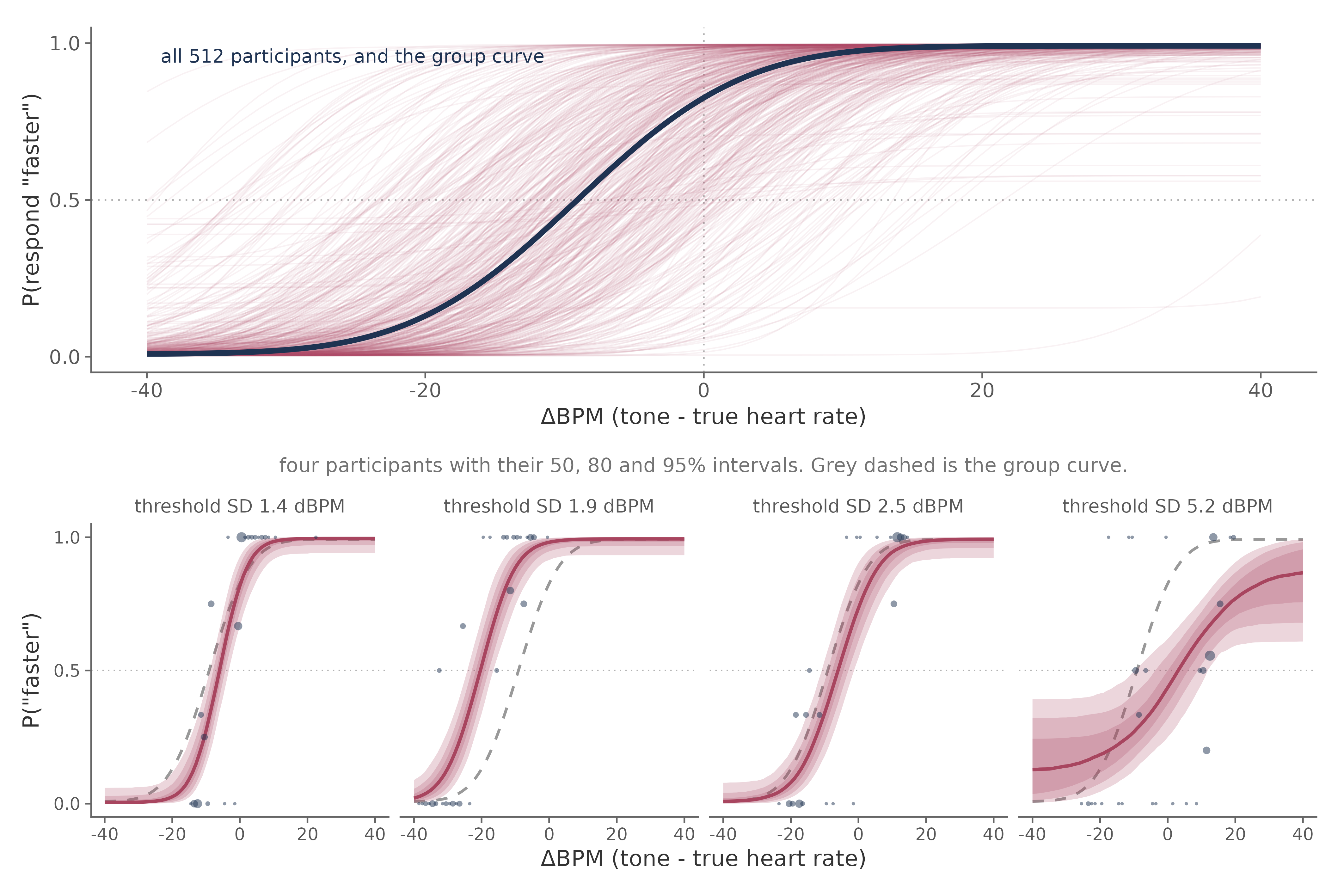
The values above the lower panels are posterior standard deviations of the threshold. They range from 1.4 ΔBPM for the first participant to 5.2 ΔBPM for the fourth. Across the full sample they range from approximately 1.1 to 17.2 ΔBPM. These numbers describe how precisely a threshold is known, not where the threshold lies.

Partial pooling also regularizes poorly constrained individual fits. Each participant is estimated mainly from their own responses, with increasing support from the population distribution as their data become less informative. Participants with clear data remain largely unchanged.

The simplest model has one population distribution and one participant-level deviation for each psychometric parameter:

bff <- bf(
  y | trials(n) ~ inv_logit(lambda) / 2 +
    (1 - inv_logit(lambda)) *
      (0.5 + 0.5 * erf(exp(beta) * (x - alpha) / sqrt(2))),
  alpha  ~ 1 + (1 | subj),
  beta   ~ 1 + (1 | subj),
  lambda ~ 1 + (1 | subj),
  nl = TRUE,
  family = binomial(link = "identity")
)

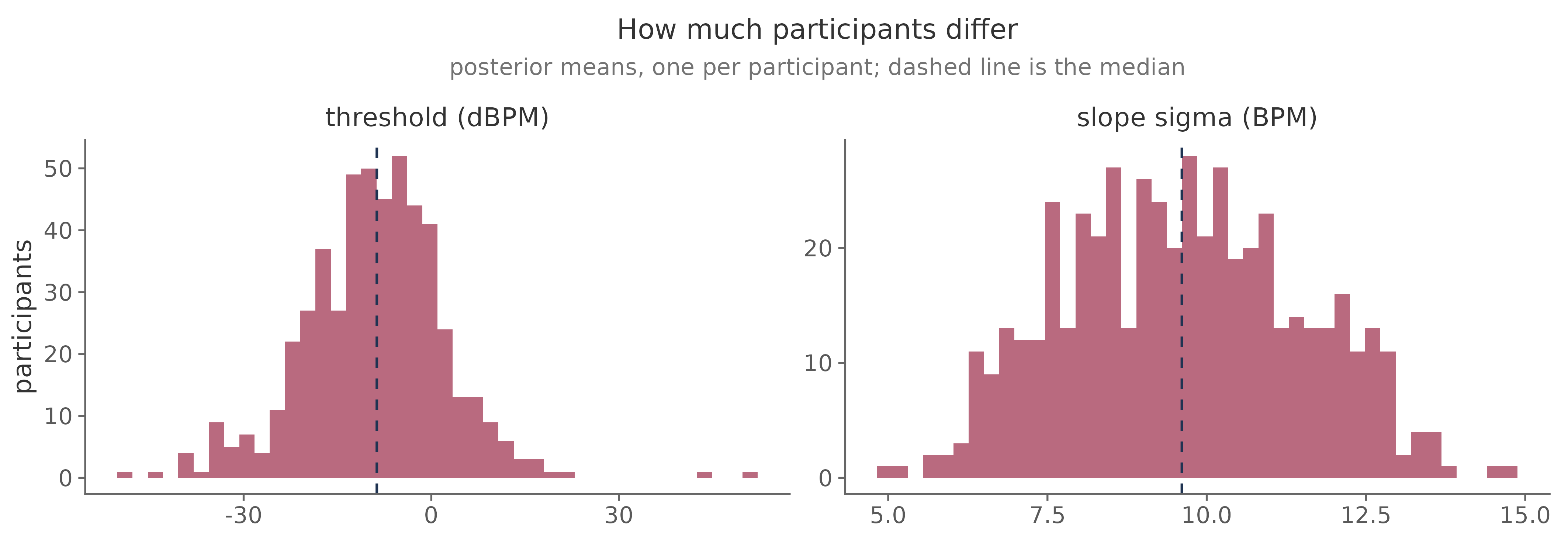
The distribution of participant posterior means gives a first impression of the heterogeneity in the sample. It is not a substitute for the posterior of the population standard deviations, which should be reported from the model itself.

Translate the design into a formula

Predictors can affect threshold, slope, or both. For the worked example we put the same design terms on alpha and beta. This allows the data to distinguish a horizontal shift in the curve from a change in its steepness. Holding one parameter fixed can force an effect into the other.

The random-effects structure follows the experimental design. A term receives a participant-level slope when it varies within participants. Modality, a pre-post contrast, and a crossover treatment meet this criterion. Gender, age, BMI, and diagnostic group do not.

Study design	Formula for alpha and beta
One condition and one group	~ 1 + (1 | subj)
Intero and Extero, pre and post, or drug and placebo	~ condition + (condition | subj)
Patients and controls, or gender	~ group + (1 | subj)
Age, BMI, or a questionnaire score	~ age_z + (1 | subj)
Covariates plus a within-participant condition	~ Modality + gender + age_z + bmi_z + (Modality | subj)
A group difference specific to interoception	~ Modality * group + (Modality | subj)

A term such as (gender | subj) asks the model to estimate how a participant’s gender changes across trials. There is no such variation. In a complex model, this error may appear as divergences or a group standard deviation close to zero rather than as a helpful error message.

Continuous covariates are centered and scaled over participants:

model_df$age_z <- as.numeric(scale(model_df$age))
model_df$bmi_z <- as.numeric(scale(model_df$bmi))

Do this using one row per participant. Scaling the trial table gives more weight to participants with more usable trials. After scaling, the intercept describes a participant at the sample mean of the covariates, and each coefficient is expressed per sample standard deviation.

The worked design

The worked dataset contains 512 participants who completed both HRD conditions. The model includes gender, age, and BMI. Modality varies within participants; the other predictors vary between participants.

alpha  ~ Modality * (gender + age_z) + bmi_z + (Modality | subj)
beta   ~ Modality * (gender + age_z) + bmi_z + (Modality | subj)
lambda ~ 1 + (1 | subj)

The interactions with Modality address a specific scientific question. They ask whether the associations with gender and age differ between judgements of the heart and judgements of the auditory control stimulus. A model containing only main effects assumes that these associations are identical in the two conditions.

That assumption may be reasonable for some studies. It should follow from the research question rather than from a preference for the shortest formula. In the worked model, BMI is included as a covariate without a modality interaction.

Treatment coding makes the auditory condition and women the reference levels. The population intercepts therefore describe an exteroceptive judgement by a woman at the sample mean of age and BMI. Every coefficient below must be read relative to that reference cell.

Choose and check the priors

The intercept and population-scale priors come from the population refit in Courtin et al. (2026). They provide useful information about plausible HRD thresholds, slopes, lapse rates, and between-participant variation.

Each additional coefficient also needs a prior. The worked analysis centers these priors on zero and scales them relative to the between-participant standard deviation of the relevant psychometric parameter:

set_prior("normal(0, 11.23)", class = "b", nlpar = "alpha",
          coef = "genderMale")
set_prior("normal(0, 5.62)", class = "b", nlpar = "alpha",
          coef = "age_z")
set_prior("normal(0, 2.81)", class = "b", nlpar = "alpha",
          coef = "ModalityIntero:genderMale")

The first prior allows a binary group contrast to be as large as the population spread in thresholds. The prior for a one-standard-deviation change in age is half as wide, and the interaction prior is narrower again. These scales are choices made for this worked example. They should not be presented as population estimates from Courtin et al.

Check that the priors correspond to coefficients generated by the formula:

get_prior(bff, model_df)

The scripts accompanying this tutorial perform this check before sampling. This is worth doing explicitly whenever the formula changes.

A prior predictive check examines what the model implies before seeing the responses:

fit_prior <- brm(
  bff,
  data = model_df,
  prior = priors,
  sample_prior = "only",
  chains = 4,
  cores = 4,
  backend = "cmdstanr"
)

Plot the implied psychometric curves and inspect the threshold distribution. A prior that places most thresholds outside the stimulus range describes effects that the experiment cannot identify.

Fit and cache the model

fit <- brm(
  bff,
  data = model_df,
  prior = priors,
  chains = 4,
  cores = 4,
  warmup = 2000,
  iter = 4000,
  control = list(adapt_delta = 0.95, max_treedepth = 12),
  backend = "cmdstanr",
  seed = 12345,
  file = "fit_hrd"
)

Always set file. A full HRD model can take hours, depending on the number of participants, the formula, the processor, and the Stan configuration. Caching prevents an accidental rerun from starting the sampler again.

Develop the pipeline on a small subset with short chains. This checks the data preparation, formula, priors, and post-processing, but it does not produce reportable estimates. Run the final model with the full dataset and planned sampling settings.

On a compute node, within-chain threading can reduce elapsed time:

fit <- brm(
  ...,
  chains = 4,
  cores = 4,
  threads = threading(2),
  backend = "cmdstanr"
)

The product of chains and threads should not exceed the number of physical cores allocated to the job.

Check the fit

We recommend checking the fit in the following order:

1. Confirm that there are no divergent transitions after warmup.

2. Check whether any transitions reached the maximum tree depth and inspect E-BFMI for each chain.

3. Confirm that all relevant rhat values are below 1.01 and that bulk and tail effective sample sizes are adequate.

4. Examine posterior predictive checks at both the participant and population levels.

5. Interpret the coefficients only after these checks are satisfactory.

Increasing adapt_delta to 0.99 can help with occasional divergences. Persistent divergences usually call for another look at the model structure and data. A random slope on a between-participant factor is one common cause.

Participant-level checks

Plot fitted curves against the observations for a range of participants. The panels below span the fitted threshold distribution rather than showing only the cleanest examples.

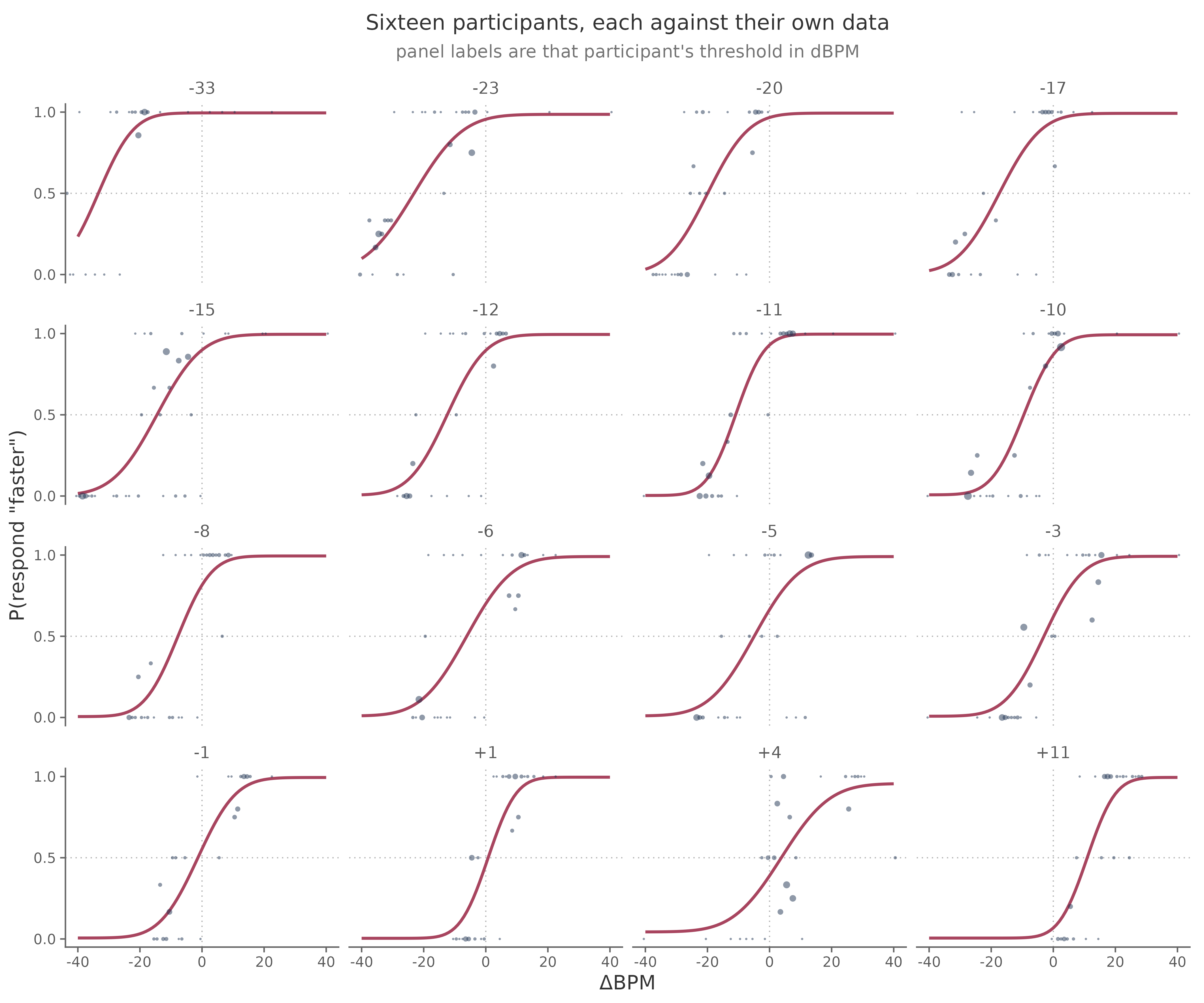
Look for systematic departures between the curve and the responses. Some participants will have wide posterior uncertainty because the staircase did not obtain enough informative trials. That is expected and should be visible.

Population-level checks

The pooled check bins the observed responses and compares them with predictions for the same participants and trials.

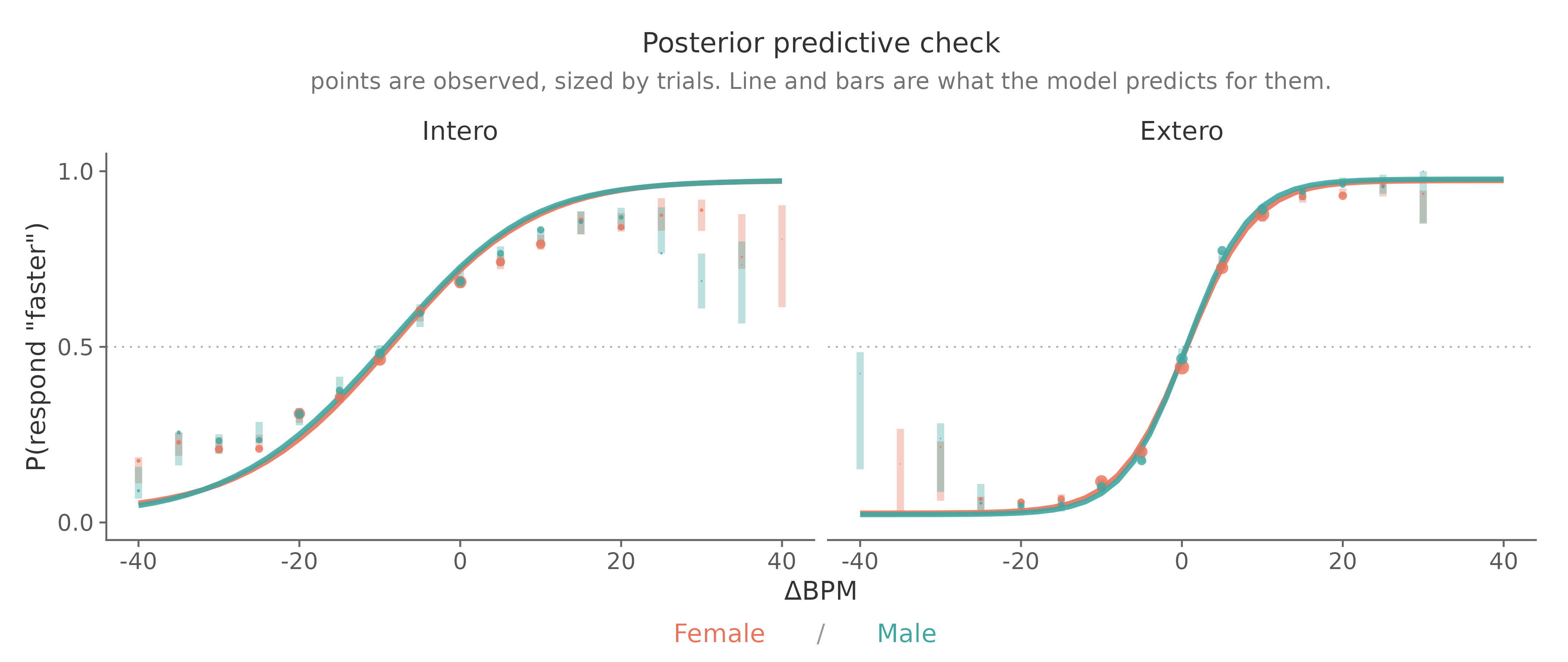
The points are observed response proportions. The line and intervals are model predictions. This is a graphical check of where the model reproduces the data; the number of bins covered by a 95% interval is not a test of model validity.

Use posterior_predict() for predictive intervals. posterior_epred() describes uncertainty in the expected response and omits binomial sampling variation. Its intervals are therefore too narrow for this particular comparison. Predictions should also retain participant effects because the adaptive staircase sends different participants to different parts of the intensity range.

Interpret the worked model

The fitted curves below show population-level predictions at the sample mean of age and BMI, separately for gender and modality.

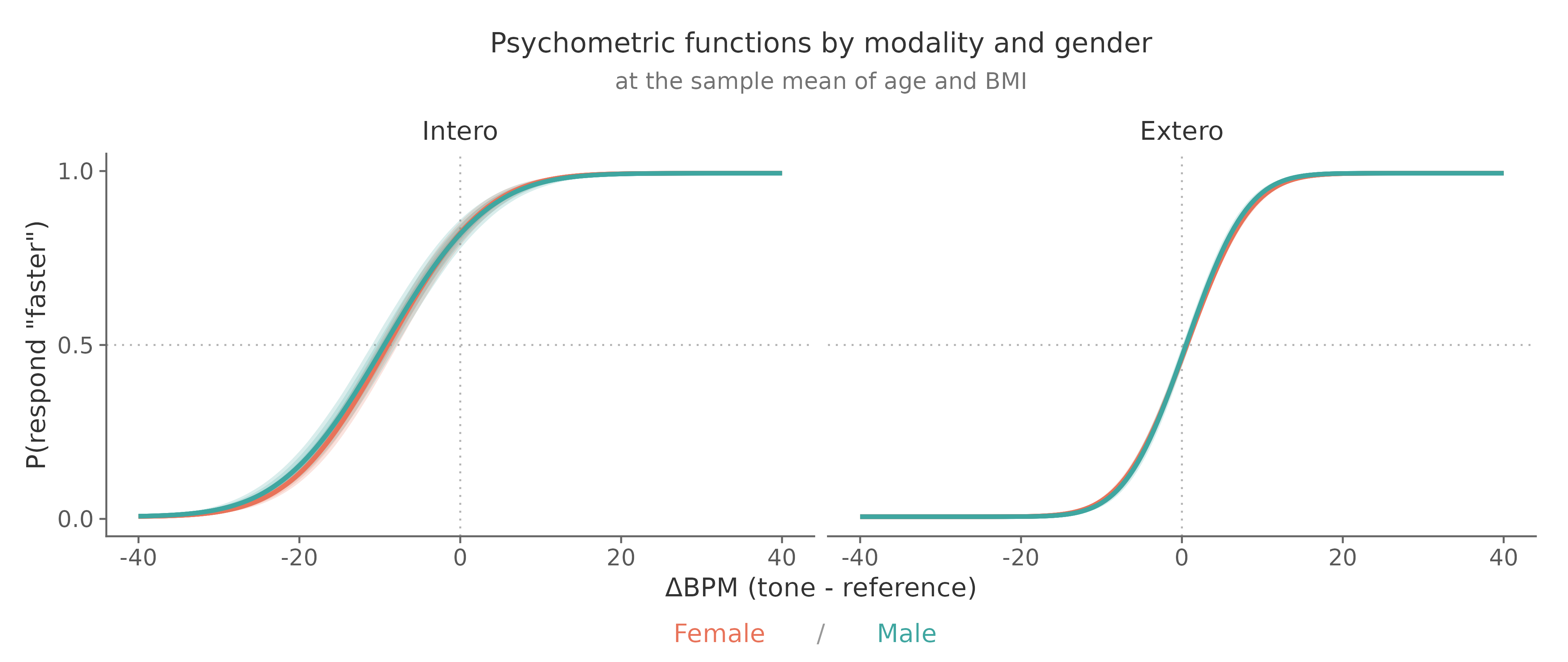
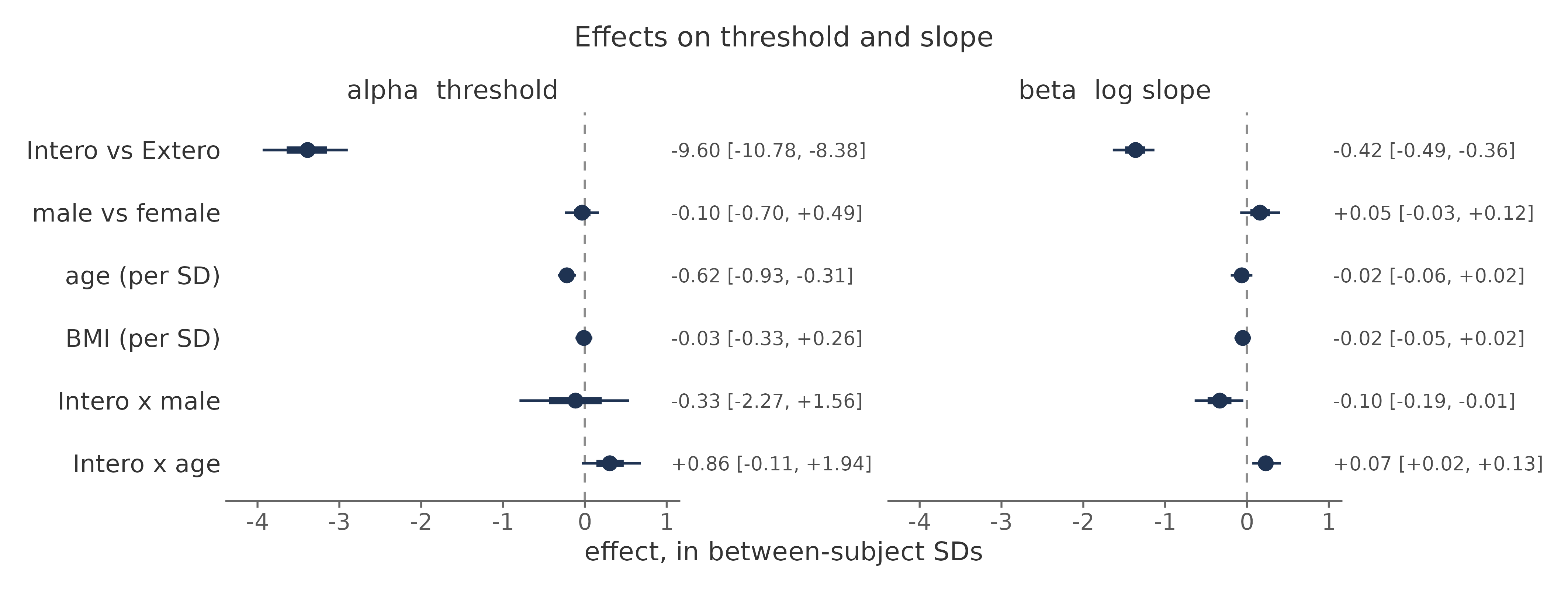
Selected coefficients from the worked model are shown below. The auditory condition and women are the reference levels.

Term	Posterior mean	95% credible interval
alpha_Intercept	+0.60 ΔBPM	[0.24, 0.97]
alpha_ModalityIntero	-9.60 ΔBPM	[-10.77, -8.37]
alpha_genderMale	-0.09 ΔBPM	[-0.69, 0.49]
alpha_age_z	-0.62 ΔBPM per SD	[-0.94, -0.32]
alpha_bmi_z	-0.03 ΔBPM per SD	[-0.33, 0.26]
beta_ModalityIntero	-0.42	[-0.48, -0.36]
beta_ModalityIntero:genderMale	-0.10	[-0.196, -0.014]
beta_ModalityIntero:age_z	+0.07	[0.020, 0.124]

For the reference participant, the estimated auditory threshold is close to zero. Adding the modality coefficient gives a cardiac threshold of about -9.0 ΔBPM. This corresponds to judging tones approximately 9 BPM below the true heart rate as equally likely to be faster or slower.

The negative modality coefficient on beta indicates a shallower cardiac psychometric function. On the more interpretable sigma scale, the fitted values are approximately 6.3 BPM for the auditory condition and 9.6 BPM for the cardiac condition. A larger sigma means poorer discrimination.

These are reference-cell estimates. Population-average statements should come from marginal predictions or contrasts averaged over the sample distribution of the covariates.

The next figure standardizes each coefficient by the corresponding between-participant standard deviation. The native-scale estimates remain printed beside the intervals.

Read interactions through simple effects

Once an interaction is present, a main-effect coefficient describes the reference condition. For example, beta_genderMale is the gender contrast in the auditory condition. The corresponding cardiac contrast is the sum of beta_genderMale and beta_ModalityIntero:genderMale.

The same rule applies to continuous covariates. alpha_age_z is the age slope in the auditory condition. The cardiac age slope is:

draws <- posterior::as_draws_df(fit)

age_effects <- draws |>
  dplyr::transmute(
    alpha_age_extero = b_alpha_age_z,
    alpha_age_intero = b_alpha_age_z +
      `b_alpha_ModalityIntero:age_z`,
    beta_age_extero = b_beta_age_z,
    beta_age_intero = b_beta_age_z +
      `b_beta_ModalityIntero:age_z`
  )

Summarize these derived posterior distributions directly. The interaction tells you how much the two condition-specific effects differ. It does not, on its own, establish that either simple effect differs from zero.

The age figure shows the same calculation on the parameter scales, averaged over the observed gender composition of the sample.

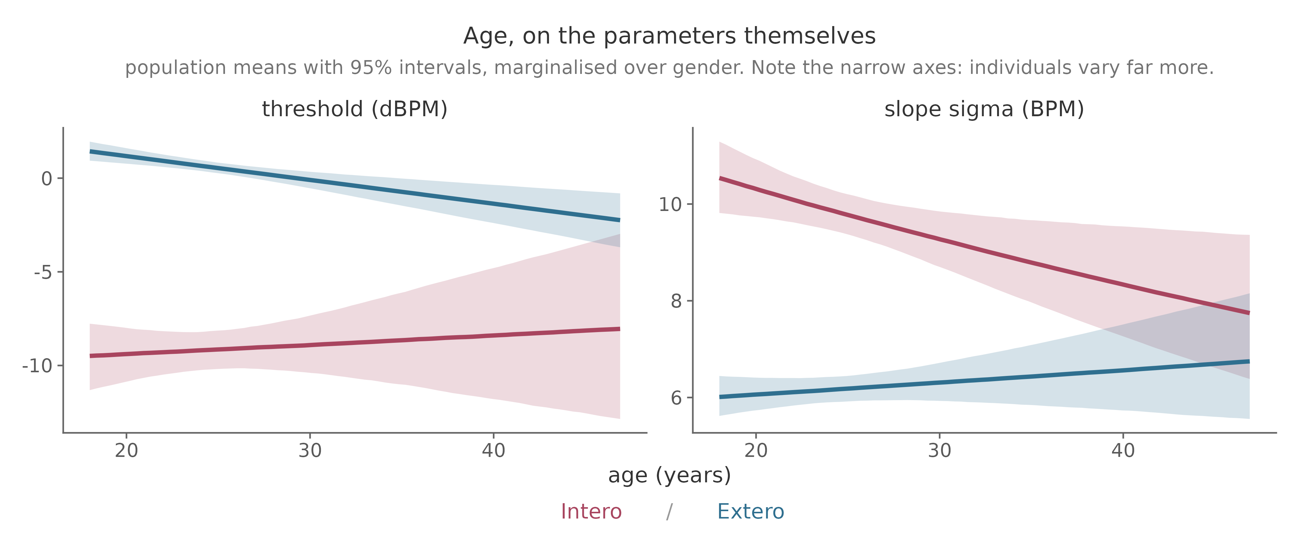
The auditory threshold decreases with age in this dataset. The cardiac trend is flatter because the modality interaction offsets much of that association. On the sigma scale, auditory discrimination changes little across age, while the cardiac curve becomes steeper. Formal claims should be based on the posterior intervals and probabilities of the simple effects calculated above.

Report the model

A report should include:

• the psychometric function and response coding;

• the formulas for alpha, beta, and lambda;

• the prior distributions and their justification;

• the number of participants, trials, and aggregated cells;

• sampler settings and diagnostics;

• posterior estimates with credible intervals;

• condition-specific contrasts when interactions are present; and

• participant-level and population-level predictive checks.

Report threshold and slope together. They describe different properties of the psychometric function, and evidence about one does not imply evidence about the other.

For a directional claim, report the posterior probability in addition to the interval:

hypothesis(fit, "alpha_genderMale > 0")
mean(posterior::as_draws_df(fit)$b_alpha_genderMale > 0)

Whenever possible, accompany latent-scale coefficients with marginal predictions or contrasts in ΔBPM and sigma. These are easier to relate to the task and less dependent on the chosen reference levels.

Population curves and pooled observations

This distinction is useful when a population curve appears not to pass through pooled observations.

The population-level coefficients describe the psychometric function of a participant whose random effects are zero. In brms, this is obtained with re_formula = NA. Pooled observations describe a different quantity: the average response across participants, each with their own threshold, slope, and lapse rate.

These quantities differ because the psychometric function is nonlinear. Averaging curves with different thresholds produces a shallower function than evaluating one curve at the average parameters.

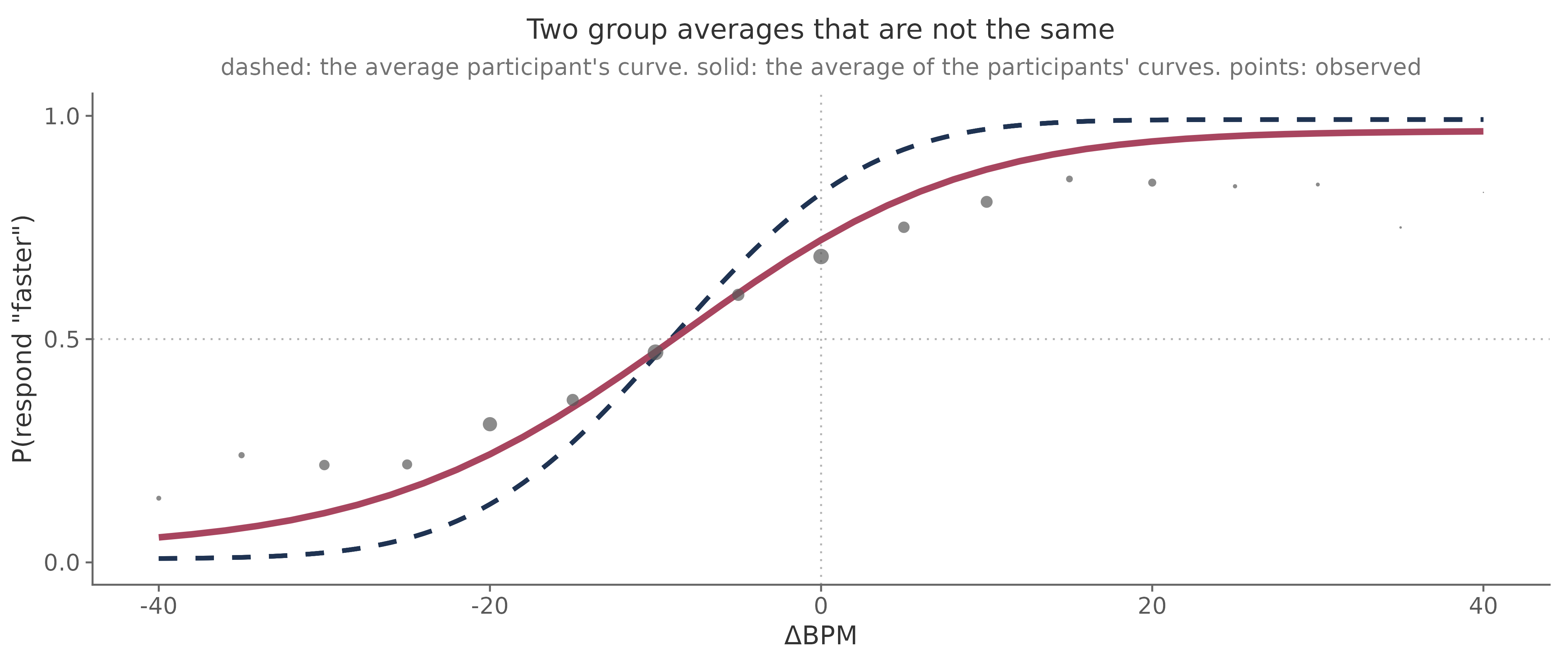
The difference is small in the auditory condition and larger in the cardiac condition, where participants vary more in threshold:

Condition	Between-participant threshold SD	Largest difference between curves
Auditory	2.44 ΔBPM	0.026
Cardiac	10.97 ΔBPM	0.099

For model checking, compare each participant with their own fitted curve, or compare pooled bins with predictions made over the participants and trials that produced those bins. Avoid comparing pooled observations with the curve of a zero-random-effect participant.

The adaptive staircase adds a second reason for care. Trials at an extreme ΔBPM tend to come from participants whose thresholds lie near that value. Those trials are not a representative sample of the population, and a prediction over the observed trial structure should preserve that selection.

Continue to the confidence model

The metacognition tutorial is the second hierarchical model in this workflow. This page modelled choices with a nonlinear binomial psychometric function. The next page models trial-level confidence with ordered beta regression, including responses at 0 and 100.

The design principles carry over. Participants receive varying effects for predictors that change within person, group-level predictors receive no participant slope, and interactions answer whether an effect differs by condition or group. The outcome and likelihood change, and so does the quantity we interpret. In the confidence model, Accuracy and its interactions describe metacognitive calibration, while the remaining main effects describe confidence bias.