HSD validation and technical details

HSD has been evaluated in simulations and a single hardware demonstration. The simulations test how well the procedure recovers known response patterns; the hardware session checks recording and stimulus delivery. Neither establishes validity as a measure of heartbeat perception in a participant population.

This page explains the main findings before presenting the detailed numerical results and development history. For the model and adaptive procedure, see HSD method and rationale. For session setup, see the task page.

Simulation study

The study examined how quickly adaptive sampling estimates preferred heartbeat timing, which response patterns are difficult to recover, and whether the evidence distinguishes a timing-dependent response from a flat one. It compared three adaptive procedures with a 120-trial method of constant stimuli (MCS).

Important

The figures and tables below report marginal estimates of \(\mu\), including the stopping analyses. The current task reports conditional timing estimates and uses their intervals for stopping. A full rerun of these results with the conditional estimates is pending. The reported stopping proportions should therefore not be treated as predictions for the current task.

The simulations included 38 observer profiles: 30 with a timing-dependent response, six with flat responses at different yes rates, and two with asymmetric response patterns. Each method was run ten times per profile for 120 trials, giving 1,520 runs per timing condition. Each trial represented a five-tone judgement.

The two timing conditions used jitter standard deviations of 26 and 6 ms, based on measurements from the test desktop and laboratory PC. Simulations also included a minimum delay, a heart-period-dependent upper limit, and trials with no delivered tones. The MCS benchmark retained its classical 0 to 500 ms delays, including delays unavailable to the adaptive task on the current hardware. The comparison therefore reflects both sampling strategy and access to different delays.

The default adaptive procedure, psi_mu_x10, targets \(\mu\) and selects a random delay on 10 percent of trials. The other adaptive procedures target \(\mu\) without exploration (psi_mu) or jointly target \(\mu\) and \(\sigma\) (psi_mu_sigma). Unless stated otherwise, accuracy summaries cover the 30 timing-dependent profiles, or 300 runs per method.

Observer profiles, comparison methods, and simulation settings

Observers.

Group	Parameters	Count
Detectors	mu in {150, 200, 250, 300, 350} ms; sigma in {50, 100, 150} ms; (floor, peak) in {(0.05, 0.95)} (clean) or {(0.2, 0.8)} (noisy)	30
Non-detectors	Flat “yes” rate of 0.3 or 0.5	2
Misspecified	Asymmetric envelope, right tail twice as wide as the left, mu at 200 or 300 ms, sigma 100 ms, (floor, peak) = (0.05, 0.95)	2
Biased non-detectors	Always “yes”, always “no”, flat 0.1, flat 0.9	4

Methods.

Label	Method
MCS	Six delays from 0 to 500 ms, 20 trials each, random order. Analyzed on the same grid posterior, and with the classical median interval and interquartile range
psi_mu	Psi-marginal, target mu; sigma, floor and peak as nuisances
psi_mu_x10	The same with explore at 0.1: the task’s default
psi_mu_sigma	Psi-marginal, target mu and sigma

Timing and delivery assumptions. Each simulated participant has a resting heart period drawn uniformly from 0.8 to 1.1 s, the same for every method. The adaptive methods present candidates from 140 ms (the first above the 130 ms floor) up to the task’s ceiling at that period, TaskConfig.bounds, which is 570 to 784 ms, so the top candidate is 560 or 600 ms. The observer answers at the nominal delay plus Gaussian timing noise, one draw per trial, while the engine is updated with the nominal delay: 26 ms SD, the Bluetooth jitter of the ECG stamps on the test desktop, and 6 ms, that of the lab PC. One draw per trial is pessimistic if the five tones of a train average out. On 7 percent of trials no train is delivered and the trial gives no update but still counts, as the dry run lost 4 of its 60 trains (though those still gave an update). Jitter and lost trains apply to MCS too, which keeps its published levels from 0 to 500 ms as the classical benchmark, although 0 ms cannot be realized on current hardware.

Replications. Ten repetitions per observer and method, seeded through the package’s random number generator so every run can be reproduced: 38 observers, 4 methods, 10 repetitions and 120 trials, 1,520 runs per study, with the seeds of the earlier studies for the first 34 observers. Each study took 37 minutes with 28 worker processes on a 32-core machine. The commands are under how to reproduce.

Metrics. Absolute error and root mean squared error of the posterior mean of mu at each trial count; credible-interval width; coverage of the 95 percent interval; error in sigma; the detection Bayes factor per observer group; the stopping rule applied to every run; the distribution of sampled delays, which is the check on clustering.

Outputs. CSVs of per-trial estimates, of summaries by trial count, of detection evidence by group and of the stopping rule, a figure of RMSE and credible-interval width against trial count by method, and a table at 15, 20, 30, 40, 60 and 120 trials. The simulation script regenerates all of them.

Accuracy of heartbeat timing estimates

Adaptive sampling reduced estimation error early in the simulated sessions. Its advantage diminished with additional trials, and MCS had lower error by 120 trials. The figure shows both estimation error and uncertainty: narrower intervals do not necessarily imply lower error.

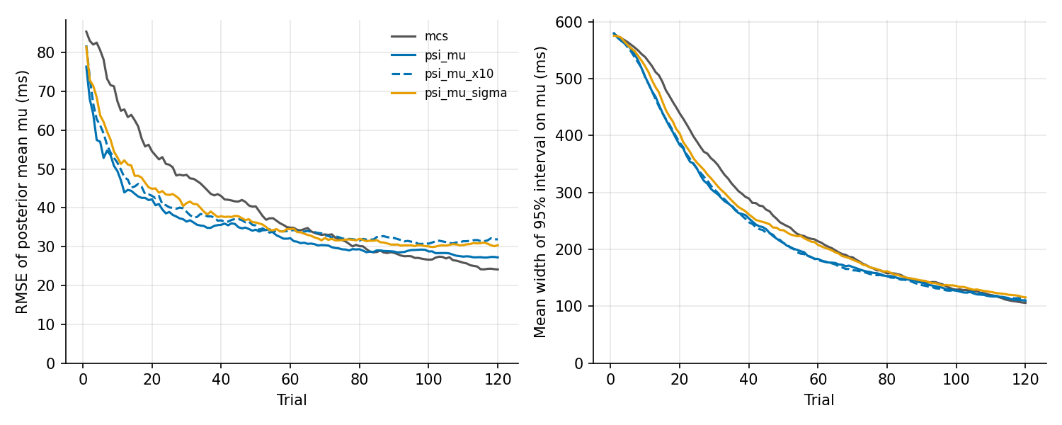
RMSE of the posterior mean of mu (left) and mean width of its 95 percent credible interval (right) against trial count, by method, for the 30 detectors, as the task runs with 26 ms of timing jitter.

For the default adaptive procedure with 26 ms jitter, root mean squared error (RMSE) was about 45 ms after 15 trials and 34 ms after 60 trials. MCS had corresponding errors of about 63 and 35 ms. By 120 trials, MCS reached about 24 ms, compared with 32 ms for the default adaptive procedure.

The advantage of MCS at longer sessions needs to be interpreted alongside its access to earlier delays. Those delays are particularly informative for participants whose heartbeat sensation occurs early in the cardiac cycle.

Detailed accuracy results

Full accuracy and interval-width results

mu RMSE (ms) at trial	15	20	30	40	60	120
MCS, 26 ms jitter	62.6	54.6	48.5	43.0	34.9	24.1
psi_mu, 26 ms	43.6	42.2	36.5	35.6	32.2	27.2
psi_mu_x10, 26 ms	45.5	43.1	39.0	36.8	34.2	31.9
psi_mu_sigma, 26 ms	48.2	44.9	41.2	37.8	34.5	30.4
MCS, 6 ms jitter	65.1	57.5	48.2	40.9	33.8	23.6
psi_mu, 6 ms	41.7	39.7	35.7	32.7	28.0	26.1
psi_mu_x10, 6 ms	44.6	39.1	35.2	32.9	30.1	26.8
psi_mu_sigma, 6 ms	43.0	38.8	35.3	33.0	31.8	27.7
Median absolute error, psi_mu_x10, 26 ms	26.4	26.9	23.4	22.1	16.3	12.6
Median absolute error, psi_mu_x10, 6 ms	24.1	23.2	19.6	17.2	14.6	9.8
Bias, psi_mu_x10, 26 ms	-4.6	-8.2	-11.6	-11.4	-12.2	-11.3
Mean CI width, MCS, 26 ms	495	439	355	290	214	106
Mean CI width, psi_mu_x10, 26 ms	440	388	305	248	181	112
Mean CI width, psi_mu_x10, 6 ms	420	367	287	234	163	95

The adaptive methods have a lower RMSE than MCS up to about trial 60 to 80, depending on the method and the jitter; by 120 trials MCS is the most accurate (24 ms against 27 to 32 ms), because its levels are not held to the floor. Inside the task’s 60 trials the gain over MCS is largest early: 45 against 63 ms at 15 trials and 39 against 49 ms at 30 (26 ms of jitter). The median absolute error of psi_mu_x10 is within the 20 to 30 ms target from 15 trials, and below 20 ms from about 40 trials with 6 ms of jitter and 60 with 26 ms. Exploration changes the RMSE by at most 3 ms within 60 trials, and costs 5 ms at 120 trials with 26 ms of jitter. Jitter of 26 rather than 6 ms costs about 4 ms of RMSE at 60 trials (34.2 against 30.1 ms for psi_mu_x10) and widens the interval by about 20 ms. On the same MCS data the classical median interval has an RMSE of 38 ms at 120 trials against 24 ms for the grid posterior.

Response patterns that are difficult to estimate

The largest location errors occurred for early sensations. When much of the rising side of the response envelope falls below the minimum delay, the task mainly observes its falling side. Several earlier values of \(\mu\) can then explain similar data, pulling the posterior mean towards earlier delays.

This explains the mean bias of about -11 ms across timing-dependent observers. It also explains why additional trials alone do not remove the error: the missing part of the response pattern remains inaccessible.

Location error by preferred delay at 120 trials

True mu	150 ms	200 ms	250 ms	300 ms	350 ms
RMSE (ms), 26 ms jitter	38.4	44.4	30.6	14.6	22.1
RMSE (ms), 6 ms jitter	36.5	30.5	28.9	17.3	14.3
Bias (ms), 26 ms jitter	-26.5	-17.0	-7.2	-2.3	-3.7
Bias (ms), 6 ms jitter	-24.5	-7.2	-9.3	+0.5	+0.2

Asymmetric response patterns introduce a different problem. The model assumes a symmetric Gaussian envelope. For the two asymmetric observers, the default procedure had an RMSE of 42 ms with 26 ms jitter and 33 ms with 6 ms jitter after 120 trials (20 runs per method). These results show the sensitivity of location estimates to the shape assumed by the model.

The marginal 95 percent intervals covered the true \(\mu\) in 96 to 100 percent of runs across methods and trial counts from 15 onward. They were conservative in these simulations. This coverage result does not establish coverage of the conditional intervals used by the current task.

Effects of timing variability

Reducing jitter from 26 to 6 ms lowered the default procedure’s RMSE at 60 trials from 34.2 to 30.1 ms and narrowed its mean interval by about 20 ms. The benefit was modest for location, but timing variability also broadens the response envelope and complicates interpretation of \(\sigma\).

Width was recovered less accurately than location under adaptive sampling. With 26 ms jitter, error in \(\sigma\) fell only from about 36 ms at 15 trials to 32 ms at 120 trials. At 120 trials it was about 27 ms with 6 ms jitter; MCS reached 21 to 24 ms. Improving hardware timing and estimating perceptual width therefore remain separate validation concerns.

Detection evidence

Detection evidence generally distinguished timing-dependent from flat responses at the group level. It did not reliably classify every simulated observer within 60 trials. Flat responders with yes rates near 0.3 or 0.5 and observers with noisy timing-dependent responses were the hardest cases.

The table reports the median base-10 logarithm of the detection Bayes factor for the default procedure with 26 ms jitter. Positive values favour a rise in response probability across the sampled delays; negative values favour the alternative. The final column shows the proportion of runs favouring a rise after 60 trials.

Group	30 trials	60 trials	120 trials	Share above 0 at 60 trials
Clean detectors	+1.45	+2.27	+3.71	1.00
Noisy detectors	+0.67	+1.36	+2.00	0.91
Asymmetric	+0.95	+1.41	+2.03	1.00
Always “yes”	-2.52	-3.97	-6.04	0
Always “no”	-1.17	-1.85	-2.85	0
Flat 0.1	-0.45	-0.90	-1.38	0
Flat 0.9	-0.68	-1.11	-1.61	0
Flat 0.3	-0.11	-0.20	-0.69	0.2
Flat 0.5	-0.00	-0.45	-0.69	0.3

After 60 trials, evidence still favoured a rise in 2 or 3 of 10 runs for the flat 0.3 and 0.5 responders. Conversely, 9 percent of noisy detector runs did not favour a rise. These errors are why the task reports detection evidence as a monitoring measure rather than a participant classification.

Comparisons across timing conditions and methods

With 6 ms of jitter the detectors’ medians are a little higher (clean +2.54, noisy +1.49 at 60 trials); the non-detectors’ answers do not depend on the delay, so jitter does not change them. psi_mu and psi_mu_sigma are within about 0.4 of psi_mu_x10 at 60 trials. MCS gives detectors larger factors from about 40 trials (clean +3.02 at 60), since its fixed levels sample both flanks and the far tail.

The Bayes factor now favours a rise for every detector group and a flat envelope for every non-detector group, the biased ones included, and it moves further with more trials in both directions. A biased non-detector is the clearest case: answering almost always “yes” or “no” puts the evidence firmly against a rise, where the old grids took it as strong evidence for one. The hard cases are non-detectors near the middle of the scale, 0.3 and 0.5, whose evidence moves slowly and is still above 0 in 2 or 3 of 10 runs at 60 trials, and noisy detectors, of which 9 percent are still at or below 0 then. So the evidence separates the groups on average but not every person within 60 trials, which is why it is reported as a sanity check and not used as a classifier.

Sampling across delays

The sampled delays covered much of the available range, with a concentration at the minimum delay for early sensations. Under psi_mu_x10 with 26 ms of jitter, 16 of the 24 candidate delays from 140 to 600 ms each receive at least 2 percent of trials, with 4 to 7 percent per delay between 180 and 340 ms. The one concentration is at the floor: 21 percent of trials at 140 ms, from 33 percent for observers with a mu of 150 ms to 8 percent for a mu of 350 ms. For early sensations the floor cuts off the rising side of the envelope, so the lowest allowed delay is the most informative one left. The longest delays, 520 to 600 ms, receive 7 percent of trials.

Session length

Longer sessions improved accuracy, but the gains beyond 60 trials were small for the default procedure. Extending the maximum to 90 trials reduced RMSE by about 2 ms while allowing 50 percent more trials. The lower delay limit continued to constrain estimates for early sensations.

The historical stopping analysis used marginal intervals. With a 100 ms width criterion, about half the clean detector runs stopped before 60 trials, whereas most noisy detectors and almost all flat responders reached the maximum. These results motivated the provisional limits, but the current conditional rule needs its own evaluation.

Historical stopping results using marginal intervals

Median 95% CI width on mu	Clean, 26 ms jitter	Noisy, 26 ms	Clean, 6 ms	Noisy, 6 ms
150 ms	37 trials	Not reached by 120	34 trials	84 trials
100 ms	61 trials	Not reached	52 trials	Not reached
80 ms	75 trials	Not reached	63 trials	Not reached
60 ms	104 trials	Not reached	80 trials	Not reached

Clean observers have a floor of 0.05 and a peak of 0.95, noisy ones 0.2 and 0.8. Over all 30 detectors the median width reaches 100 ms at trial 89 with 26 ms of jitter and at trial 75 with 6 ms. Width grows with sigma: at 60 trials and 26 ms of jitter the clean medians are 60, 95 and 130 ms for a sigma of 50, 100 and 150 ms.

The historical rule was applied to each run using marginal intervals; a lost train did not count towards minTrials:

psi_mu_x10	26 ms jitter	6 ms jitter
RMSE of mu over all detectors at 15, 60 and 90 trials	45.5, 34.2, 32.3 ms	44.6, 30.1, 28.1 ms
Clean detectors stopping before 60 trials	55 percent; median stop at 55; RMSE at the stop 24.5 ms	63 percent; 48; 20.6 ms
Noisy detectors stopping before 60 trials	23 percent; RMSE at the stop 43.1 ms	31 percent; 38.8 ms
The same with maxTrials 90, noisy detectors	37 percent; 41.4 ms	45 percent; 37.0 ms

These results informed the provisional defaults. Raising maxTrials to 90 would let the median detector reach the 100 ms interval, but it lowers the RMSE of mu by only 2 ms (34.2 to 32.3 ms, and 30.1 to 28.1 ms), at 50 percent more session time: what remains is mostly the bias of the 130 ms floor for early sensations and the noise of the noisy observers, which more trials of the same kind do not remove. A 100 ms width lets about half the clean detectors stop early, at an RMSE of about 20 to 25 ms. minTrials never binds: at 15 trials the median width is still 370 to 530 ms. It stays as a guard. The non-detectors run to the maximum (239 of their 240 runs per jitter level), because the flat part of their posterior spreads mu over the whole grid.

Hardware dry run

On 2026-11-03, a single 60-trial session tested the full procedure with a PLUX ECG streamed over Bluetooth into LSL. LabRecorder recorded the ECG and HSD markers. The participant wore a tight finger pulse oximeter to provide a clear pulse sensation. This was a check of the task and recording system, not a validation study of heartbeat perception.

The session lasted 7 minutes. It delivered 290 tones during the saved trials, with no dropped ECG samples. Beat detection agreed closely with offline R-wave detection. However, variation in Bluetooth arrival timestamps remained an appreciable source of timing error.

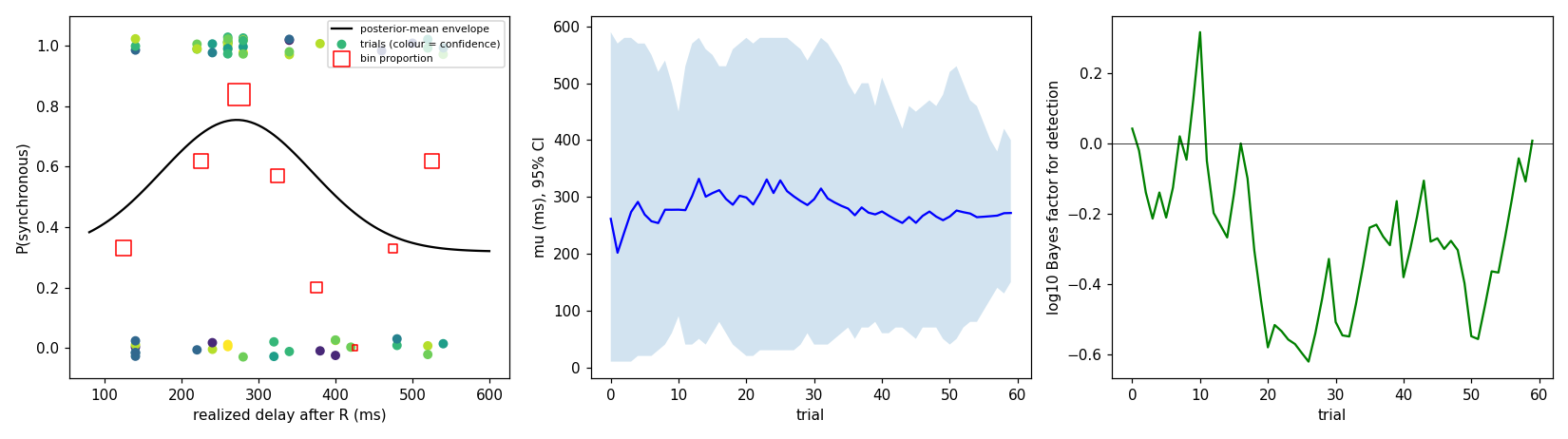
The dry run session. Left: each answer against the realized delay, coloured by confidence, with the proportion of “synchronous” answers in each 50 ms bin (squares, sized by the number of trials) and the posterior-mean envelope. Middle: posterior mean of mu and its 95 percent credible interval after each trial. Right: log10 Bayes factor for detection after each trial. All three show the posterior as the session computed it, with the old floor and peak grids.

The figure shows the session’s original estimates, calculated with earlier floor and peak grids. Responses were most often synchronous near 250 to 300 ms, but there were also frequent synchronous responses at long delays. The model therefore had limited evidence for a single, well-localized response envelope.

Re-analysis with the shared floor and peak grid left the estimated location almost unchanged, at 273 ms, while widening its marginal credible interval to 40 to 550 ms. A flat response pattern could explain the observations nearly as well. This illustrates why a plausible location estimate must be interpreted alongside detection evidence and model uncertainty.

Recording checks and timing measurements

Check	Measured
Session	60 trials in 7 minutes
Tones	290 delivered on the 60 saved trials; 6 skipped because their beat was known too late; 4 trains ended short (one ran out of beats, three reached the ceiling). The player handled 305 tones in all, the 15 of the practice trials included, which are not saved. Every reported start within 1 ms of its schedule
Online R detector	Commits a beat 13 ms (median) and 14 ms (95th percentile) after the stamped R-wave
Beat polled after its stamped R-wave, beats of a train	12 ms median, 48 ms at the 95th percentile, 63 ms at the 99th; 107 of all 506 beats polled before their stamped time, which the dejitter smooths
ECG stream	No dropped samples
Online beats against offline R-waves from the recording	Sensitivity 0.996, positive predictive value 1.0
Realized delay against the stamped R-wave	50 ms below the request on every trial, by design (the latency bias). It is taken from the scheduled start, so it checks the bookkeeping, not the sound
Tone onsets against the offline R-wave	Interquartile range of 23 ms on the raw LSL timestamps, 44 ms on the dejittered ones
Bluetooth arrival jitter of the ECG samples	SD 26 ms on the test desktop, against 6 ms on the stimulus PC

Every tone’s reported start was within 1 ms of the time it was given. The reported start is the scheduled one, so this shows that no tone started late, not when the sound came out; the offline comparison is the check on that. The scatter against the offline R-wave comes from before the scheduler. The online detector times each R-wave from the timestamps its samples carry when they arrive, and on that desktop the Bluetooth arrival times jittered with an SD of 26 ms, against 6 ms on the stimulus PC. Against the recording’s dejittered timestamps, which are closer to when the hub took each sample, the tones therefore scattered more widely (44 ms) than against its raw ones (23 ms). Jitter of this size widens the measured sigma, which is what roadmap items C2 and C3 address.

Original estimates, response counts, and re-analysis

After 60 trials, the session’s maximum, the posterior put mu at 272 ms with a 95 percent credible interval of 150 to 400 ms, sigma at 98 ms, the floor at 0.32 and the peak at 0.75. The log10 Bayes factor for detection was about 0. The interval never came down to the 100 ms stopping width, so the session ran to its maximum.

Realized delay (ms)	100 to 150	150 to 200	200 to 250	250 to 300	300 to 350	350 to 400	400 to 450	450 to 500	500 to 550
P(synchronous)	0.33	none	0.62	0.84	0.57	0.20	0.00	0.33	0.62
Trials	9	0	8	19	7	5	1	3	8

The answers rise to a clear peak at 250 to 300 ms and fall away by 350 to 400 ms. But the participant also answered “synchronous” on 5 of the 8 trials at 500 to 550 ms. The model has one bump, so it absorbed those long-delay answers as a high floor, 0.32, rather than as a second rise. A floor that high leaves the envelope a rise of only 0.43 from floor to peak, and the posterior mass on a rise of more than 0.2 stayed at 0.92, the same as its prior on those grids. That is why the Bayes factor stayed near 1 even though mu was located. Whether the long-delay answers were heard against the next beat, the periodicity the model ignores, cannot be told from one session.

Re-analyzed with the shared floor and peak grid and the rise measured over the delays presented (140 to 540 ms), the same 60 answers give mu at 273 ms but a credible interval of 40 to 550 ms, sigma at 82 ms, the floor at 0.42 and the peak at 0.76, a detection evidence of 0.70 against a prior of 0.49, and a log10 Bayes factor of +0.38. A flat responder answering “synchronous” on about 6 trials in 10 is now on the grid and explains these answers nearly as well as a rise, so about 0.3 of the posterior stays on an envelope that does not rise, spread over every mu. The location is the same; the session is weaker evidence for it than the old interval said.

What comes next

The remaining work concerns both delivery and measurement. Audio calibration and improved ECG timestamps could reduce the minimum delay and timing jitter. An exteroceptive validation task with known stimulus timing would test the procedure against a controlled reference. Validation in participants is still needed before interpreting HSD estimates as established measures of heartbeat perception.

The roadmap below records implemented components, proposed hardware changes, and their expected effects. Proposed improvements are not results from the current implementation.

Implementation status and validation roadmap

Phase	Status	Content
B. Task runner	Implemented	The task, its parameters and configuration, English instructions, an autopilot observer, the train scheduler with both stimulus axes, a headless test on a virtual heart, an LSL test on a synthetic ECG through LSLRecorder and the shared LSLBeatSource, the wrapper and the HSD page. setup="behavioral" uses the shared LSLBeatSource and TonePlayer in cardioception.devices
B. Hardware dry run	Done, 2026-11-03	The PLUX-to-LSL bridge installed on the test desktop and 60 trials run on a real ECG in 7 minutes, recorded with LabRecorder. 290 tones were delivered on the 60 trials (6 skipped as late, 4 trains short), every reported start within 1 ms of its schedule, the detector committed 13 ms after each R, no samples were dropped, and the realized delay sat 50 ms below the request by design. Against the offline R-wave the tones scattered with an interquartile range of 23 to 44 ms, because the Bluetooth arrival stamps of the ECG samples jitter (SD 26 ms on that desktop, 6 ms on the stimulus PC). The session put the sensation of a participant wearing a tight finger pulse oximeter at 272 ms, interval 150 to 400 ms. See hardware dry run
C1. Audio lead and output calibration	Planned, software only	Cut the audio scheduling lead from 50 to 20 ms (the bench showed 20 ms still lands within 1 ms) and measure the output offset of the speaker or headphones with the microphone loopback in bench/audio_onset.py, so the latency bias becomes a measured constant per setup. Lowers the physical floor from 130 to about 100 ms and makes mu comparable across laboratories
C2. Re-time PLUX samples from the hub’s counter	Planned, bridge change shared with PAT	The hub samples at exactly 1000 Hz, so a running fit of its sample counter to the clock in the bridge removes the Bluetooth arrival jitter down to the chunk period, about 10 ms, without touching the constant lag. Jitter is the error that inflates sigma: 26 ms of it turns a true width of 40 ms into a measured 48 ms. In the simulations as the task runs, 6 rather than 26 ms of jitter lowers the RMSE of mu at 60 trials from 34 to 30 ms
C3. Wired ECG into LSL	Recommended configuration	Biopac, ADInstruments and Brain Products all have LSL paths. Jitter falls to a millisecond or two, the transport lag to a few milliseconds, and with the shorter lead the floor to about 60 ms. In the earlier exact-delivery simulations an 80 ms rather than a 130 ms floor lowered the RMSE of mu at 120 trials from 26 to 17 ms and removed a 10 ms bias, because sensations at 150 to 200 ms regain their rising flank
D. Exteroceptive validation	Not started	The same adaptive procedure on a tone and vibration (or light) stimulus with a known delay, as a screening condition and as a ground-truth check of the engine

Technical details and development history

These sections preserve the measurements and earlier analyses behind the current design. Historical results should be interpreted using the settings specified for each analysis.

Timing measurements

Reported delays, latency correction, and hardware limits

Realized delays. The posterior is updated with the realized delay rather than the request: the mean over the trial’s tones of the start time the tone player reports, against the stamped R-wave, with the latency bias below added back. The likelihood is recomputed from the envelope, so any real-valued delay can be used, without requiring the delivered delay to match a point on the candidate grid. With PsychToolbox audio the reported start is the time the device scheduled, not a measurement of the sound, so the realized delay differs from the request only when a tone started late. It is not what the participant heard. The delay of each reported onset relative to an offline R-wave can be checked in the LabRecorder file (bench/pat_dryrun_report.py --markers HSD).

Delay limits. Each trial can restrict the candidates:

Limit	Set by	Why
min_delay	The system’s R-to-tone latency	No tone can be scheduled before the system knows about the R-wave. 130 ms of physical delay on current hardware (below), so 140 ms is the shortest candidate presented
max_delay	0.75 of the anticipated interbeat interval, less a 10 percent margin: about 0.68 of it on the absolute axis	Keeps the last tone clear of the next beat. The envelope is periodic in the cardiac cycle and the model ignores that, so delays near the next beat would be misread. 600 ms is allowed only at periods over 0.89 s

If no candidate lies between the two limits, the engine raises an error rather than presenting a delay outside them.

The latency floor on current hardware. These figures come from measurements on the pat-ecg branch, 2026-11-03, with a PLUX ECG streamed over Lab Streaming Layer to the stimulus PC. They are bench measurements, not a published result.

Stage	Measured
Online R detector (OnlineRDetector) commits a beat	14 ms median, 18 ms maximum after the R peak
Whole chain knows about a beat	20 ms median, 31 ms at the 95th percentile, after the R-wave
Tone scheduled with psychtoolbox audio, latency class 1, 50 ms lead	Lands within 1 ms of the scheduled time (latency class 3 was unusable on that laptop)
Dry run, tones anchored on the real R-wave	Within 17 ms of the intended phase at the 95th percentile

The latency bias. Two delays do not appear in any recording. The PLUX Bluetooth transport delivers each sample 20 to 40 ms after the hub took it, and LSL stamps it on arrival, so the stamped R-wave is late. The sound leaves the speaker some milliseconds after the onset the audio driver reports. Together these come to a roughly constant 30 to 70 ms, which the PAT dry run measured. As the PAT task does, the runner subtracts a latency bias, TaskConfig.latencyBias (50 ms by default), from every tone’s target, so that the tone reaches the participant at the requested delay after the true R-wave. A delay measured against the stamped R-wave is then 50 ms short of the physical one, and the runner adds the bias back before it updates the posterior. Both values are saved: RealizedDelay against the stamped R-wave, RealizedCorrected as the engine saw it. Both come from the start time the player reports, which is the scheduled time, so on the absolute axis RealizedCorrected equals RequestedDelay unless a tone started late (within 0.3 ms on every trial of the dry run). The phase axis applies the same subtraction to the target and the same addition to the realized fraction.

The latency floor. A tone for a physical delay d is due at the stamped R-wave plus d less the 50 ms bias. It can be scheduled only if that is at least the 50 ms audio lead after the beat is known, which on the bench was up to 31 ms (95th percentile) after the stamped R-wave. So

\[d \geq 31 + 50 + 50 = 131 \text{ ms},\]

and the runner’s floor, TaskConfig.minDelay, is 130 ms. The candidates still start at 80 ms; the per-trial bounds leave out those under the floor, so the shortest delay presented is 140 ms.

The hardware dry run measured a longer lag. Among the beats of a train, the poll that returned a beat came 12 ms (median), 48 ms (95th percentile) and 63 ms (99th percentile) after its stamped R-wave, and 107 of the session’s 506 beats were polled before their own stamped time, because the LSL inlet’s dejitter smooths the stamps. With that lag the floor would be about 150 to 165 ms, and 6 of the dry run’s tones at 140 ms were skipped because their beat was known too late. minDelay should therefore be set from the lag a session’s setup actually shows. It is left at 130 ms here. Shorter delays are possible only by scheduling predictively from the anticipated interbeat interval (the mean of the last three RR intervals). That adds the beat-to-beat variability of the heart period to the delay as jitter, and is not implemented. A sensation earlier than 130 ms can still be located, but only from the falling side of the envelope.

The simulations run at this 130 ms floor (see results as the task runs). The floor costs accuracy for sensations at 200 ms and earlier.

The latency bias is an estimate. The LabRecorder file supports an offline timing check: with the ECG and the tone markers on one clock, the offline R-waves and the reported onsets show the delay actually delivered, less the speaker.

Earlier floor and peak grids

Why the response-probability grids were revised

An earlier version had a floor grid of 0 to 0.4 and a peak grid of 0.5 to 0.97. It could express a flat responder only at rates of about 0.3 to 0.6, and explained any other non-detector as a rise. In 60 trials of the task’s configuration (bounds 130 to 514 ms, explore 0.1, three seeds), the log10 Bayes factor for detection was:

Responder	Old grids	Shared grid, rise inside the range
Always “yes”	+10.3	-4.3
Always “no”	+8.8	-2.0
Flat 0.9	+4.1 to +7.4	-1.9 to -0.5
Flat 0.1	+2.8 to +4.3	-1.5 to -1.1
Flat 0.5	-0.8 to -0.6	-0.7 to -0.2
Detector, mu 250 ms, sigma 50 ms, floor 0.1, peak 0.9	+1.6 to +2.5	+2.2 to +2.7

The biased non-detectors favoured a rise more strongly than the detector did. The estimate of mu for a detector was not affected.

Conditional estimates

The current estimation rule is explained on the methods page. The following small demonstration was recorded separately from the full simulation study.

Preliminary comparison with marginal intervals

With the task’s configuration at a 0.6 s period, a simulated observer with mu of 250 ms and sigma of 40 ms reaches a conditional interval of 70 to 170 ms after 12 trials (three seeds), compared with a marginal interval of 160 to 420 ms. The main simulation tables report marginal estimates of mu; a rerun using conditional estimates is pending.

The reported ranges need confirmation against the original output before they can be interpreted as interval widths or endpoints. They are retained here as a development record.

Earlier runs without jitter or ceiling

Exact-delivery studies and the pending control

The first studies delivered every delay exactly, had no ceiling and lost no trains, and used the old floor and peak grids. One ran 7 methods at an 80 ms floor (2,380 runs), the other 4 methods at the 130 ms floor (1,360 runs). With exact delivery, psi_mu reached a mu RMSE of 25 ms at 60 trials and 17 ms at 120 with the 80 ms floor, against 29 and 26 ms with the 130 ms floor, where a bias of about -10 ms appeared. The runs above add the ceiling, the jitter and the lost trains, and the new grids; the 6 ms run is close to the old 130 ms one (psi_mu_x10 30.1 against 30.3 ms at 60 trials), while the intervals are wider (163 against 142 ms for psi_mu_x10 at 60), because a flat envelope keeps some posterior mass spread over every mu. The earlier runs also reported that the detection evidence “moves in the right direction for both groups”; with the old grids that held only for the flat 0.3 and 0.5 responders they tested.

A control with the new grids and exact delivery at the 130 ms floor, no jitter, no ceiling and no lost trains, is pending. It would separate the effect of the new grids from that of the realistic delivery, and will be run on the cluster.

Literature checks still outstanding

Claims excluded from the design rationale

Two figures that circulate in summaries of this literature are not used on this page, because we could not open the papers to check them.

• Detector rates of 13, 43 and 47 percent for one, five and ten tones per trial, attributed to Brener, Ring and Liu [Brener et al., 1994]. The review confirms only that five tones per trial did not impair reliability relative to ten.

• A study by Schneider, Ring and Katkin [Schneider et al., 1998] said to have shifted the delay range from 0 to 500 ms to 100 to 600 ms and found that preferred delays did not move. We cite the paper only as a validity test of the MCS, which is what its title describes.

The design does not depend on either claim.

How to reproduce

The commands below record the settings used for the reported studies and a planned control. Reproducing the historical tables requires the source revision that produced their marginal estimates. The current simulation code uses conditional estimates, so running the same commands on a newer revision is not an exact reproduction of these tables.

Commands, seeds, and output files

From the repository root, at the commit that added these results, with the study seed 2026. The first two are the runs reported above; the third is the pending control.

python -m cardioception.HSD.simulate --out <dir>/jitter26 --reps 10 --processes 28 --trials 120 --seed 2026 --min-delay 130 --jitter-sd 26 --train-loss 0.07 --period 0.8 1.1 --methods mcs psi_mu psi_mu_x10 psi_mu_sigma
python -m cardioception.HSD.simulate --out <dir>/jitter6 --reps 10 --processes 28 --trials 120 --seed 2026 --min-delay 130 --jitter-sd 6 --train-loss 0.07 --period 0.8 1.1 --methods mcs psi_mu psi_mu_x10 psi_mu_sigma
python -m cardioception.HSD.simulate --out <dir>/exact130 --reps 10 --processes 28 --trials 120 --seed 2026 --min-delay 130 --jitter-sd 0 --train-loss 0 --no-ceiling --methods mcs psi_mu psi_mu_x10 psi_mu_sigma

Each writes trials.csv, summary.csv, evidence.csv, stopping.csv, delays.csv, figure.png and table.md. The figure on this page is the figure.png of the first. The run seeds do not depend on --processes, so a cluster run with a different worker count reproduces the same runs.

References

Full citation details are on the references page.